install.packages("devtools")
devtools::install_github("PATH-Global-Health/PATHtools")Installing the PATHtools package
This process uses an R package developed by PATH. This package is hosted on Github, so we have to use the devtools package to install it (you may need to install this package first).
The primary function in this package that we will use is define_urban(), which defines rural and urban areas based on population density.
The function requires a population density raster which is a gridded population surface, representing population distribution. We will download this from the GRID3 data repository.
Downloading GRID3 population rasters
We will use Senegal as an example - the download links for other countries with GRID3 population data avaliable can be found in the code block below for reference.
#  Sierra Leone: https://wopr.worldpop.org/download/473
#  South Sudan: https://wopr.worldpop.org/download/344
#  Mozambique: https://wopr.worldpop.org/download/237
#  DRC - Kinshasa, Kongo-Central, Kwango, Kwilu, and Mai-Ndombe provinces: https://wopr.worldpop.org/download/113
#  DRC - Haut-Katanga, Haut-Lomami, Ituri, Kasaï, Kasaï Oriental, Lomami and Sud-Kivu provinces: https://wopr.worldpop.org/download/488
#  Niger: https://wopr.worldpop.org/download/511
#  Burkina Faso: https://wopr.worldpop.org/download/515
#  Nigeria: https://wopr.worldpop.org/download/495
#  Zambia: https://wopr.worldpop.org/download/25
First we load some useful packages for working with rasters and shapefiles, then we will download the populaiton raster file for Senegal. The GRID3 population raster is at a resolution of 100m so we need to use the aggregate() function from the terra package to combine grid cells to a spatial resolution of 1km grid cells for input into the define_urban() function.
library(raster)        # Raster package
library(terra)         # Terra package
library(exactextractr) # exactextractr package
library(sf)            # Shapefile package
library(CHWplacement)  # CHWplacement pakacge
library(tidyverse)     # Tidyverse
library(tidyterra)     # Tidyverse methods for terra objects
library(ggforce)       # ggforce package for facet zooming
library(PATHtools)     # PATHtools package for retriving shapefiles
library(fs)            # file system package

# Load reference shapefile
shp <- PATHtools::load_shapefile(country = "Senegal", admin_level = 1)

# Grid3 raster URL
url <- "https://wopr.worldpop.org/download/502" # url for Senegal raster

# Create a temporary folder for downloaded raster
dest <- tempdir()

# file name
file_name <- fs::path(dest, "grid3-pop-raster.tif.gz")

# download and unzip the raster file
utils::download.file(url = url, destfile = file_name, mode = "wb", quiet = TRUE)
R.utils::gunzip(file_name)

# load raster into R session
population_100m <- terra::rast(fs::path(dest, "grid3-pop-raster.tif"))

# aggregate population raster from 100m grid cell resolution to 1km grid cell resolution
population_1km <- terra::aggregate(population_100m, fact=10, na.rm=TRUE, fun = "sum")

# plot population per km
ggplot() +
  geom_spatraster(data = population_1km) +
  scale_fill_whitebox_c(palette = "deep", direction = -1) +
  theme_grey() +
  labs(title = "GRID3 population per 1km Senegal 2020", fill=" ") +
  facet_zoom(xlim=c(-17,-17.6), ylim=c(14.5,15), horizontal = TRUE, shrink=TRUE, zoom.size =0.8) +
  theme(axis.text = element_blank(),
        axis.ticks = element_blank(),
        panel.grid = element_blank())
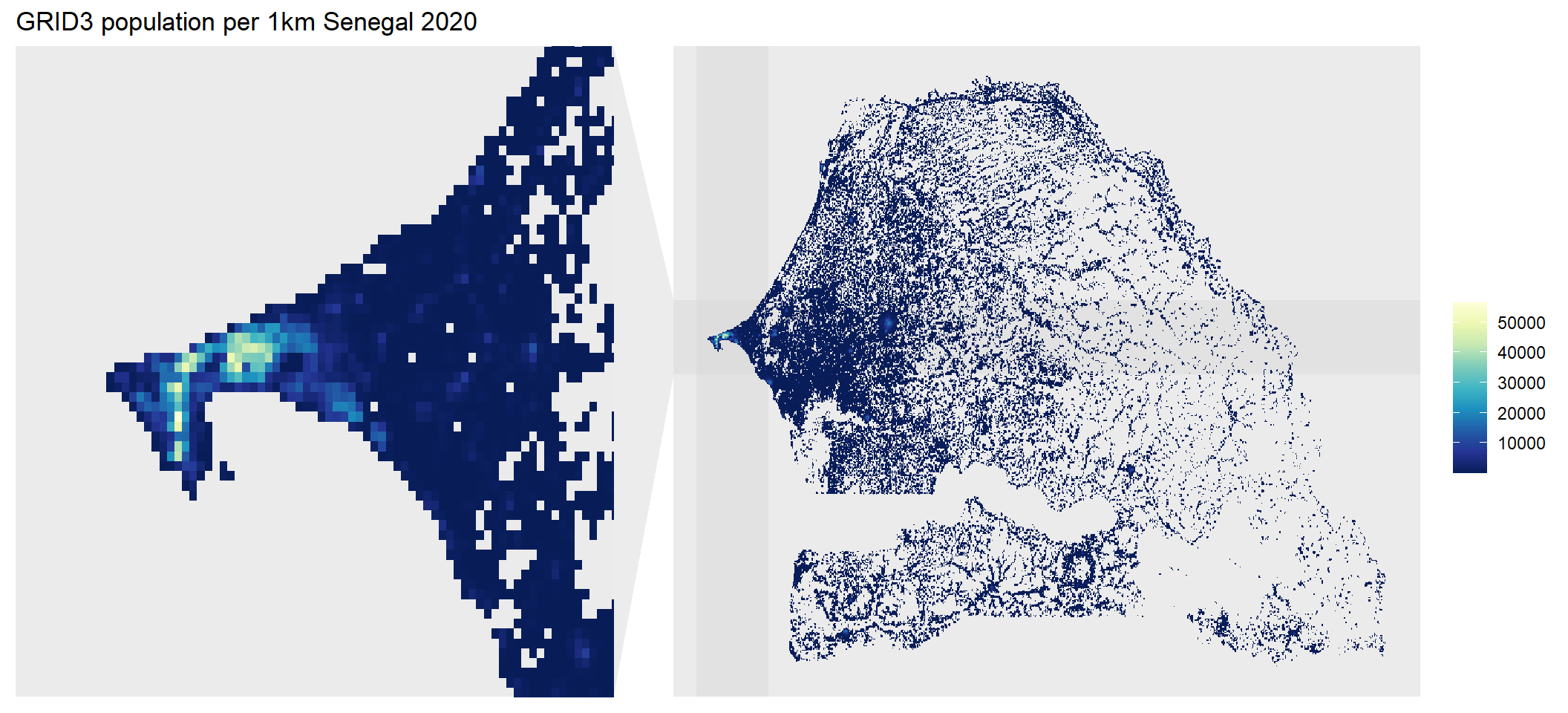
The resulting plot displays the populated areas of Senegal with those areas in yellow representing the most densely populated areas with the panel highlighting Dakar - the capital city of Senegal.
In this example I created a temporary folder (using the tempdir()) and saved it’s “path” into an object called dest. This is where we will download rasters. You can swap tempdir() with a file path to a location on your computer. Or directly read in a raster if it is already avaliable on your computer.
Classification of urban and rural areas
The next step in this work is to use the define_urban() function from the PATHtools pacakge to define urban areas. This is done using 1km² grid cells, classified according to their population density, population size and contiguity (neighbouring cells).
This function requires 3 inputs:
population_raster: An input raster containing people per pixel. Default inputs assume input resolution to be approximately 1km² resolution
rururb_cutoff: indicates the minimum population per pixel to be eligible for urban classification
min_urbsize: indicates the minimum population in the total area of contiguous selected pixels to be considered as urban
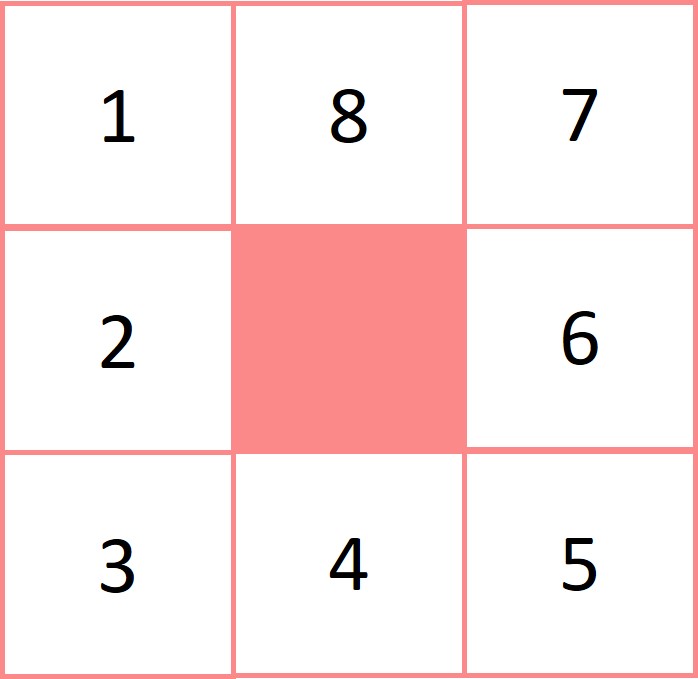
The identification of urban areas then occurs in two steps, first all cells with a population density of over runurb_cutoff are selected and then groups of contigious cells are identified using eight-point contiguity, in other words, including diagonals (see margin figure). Contigious cells are grouped together and each group with a collective population size of over min_urbsize are defined as urban.
For this example we use a population density threshold of 300 people per square km (rururb_cutoff) and a minimum population size (min_urbsize) of 10,000 people.
These values were selected based on the smallest population density threshold used to define an urban area from the Level 1 definitions in Eurostat: Applying the Degree of Urbanisation — A methodological manual to define cities, towns and rural areas for international comparisons — 2021 edition and the value of 10,000 came from the national definition of an urban area as listed in the UN Demographic Year Book 2021.
# run function to define urban clusters

# this first function call we set mask == FALSE to output a raster with only urban cells and their associated population values
ur_population <- define_urban(population_1km, min_urbsize = 10000, rururb_cutoff = 300, mask = FALSE)

# this second function call we set mask == TRUE to output a raster that defines each pixel as urban (1) or rural (0)
ur_categories <- define_urban(population_1km, min_urbsize = 10000, rururb_cutoff = 300, mask = TRUE)
cls <- data.frame(id=c(1, 0), urban_rural=c("urban", "rural"))
levels(ur_categories) <- cls
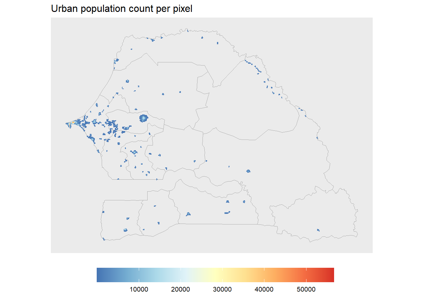
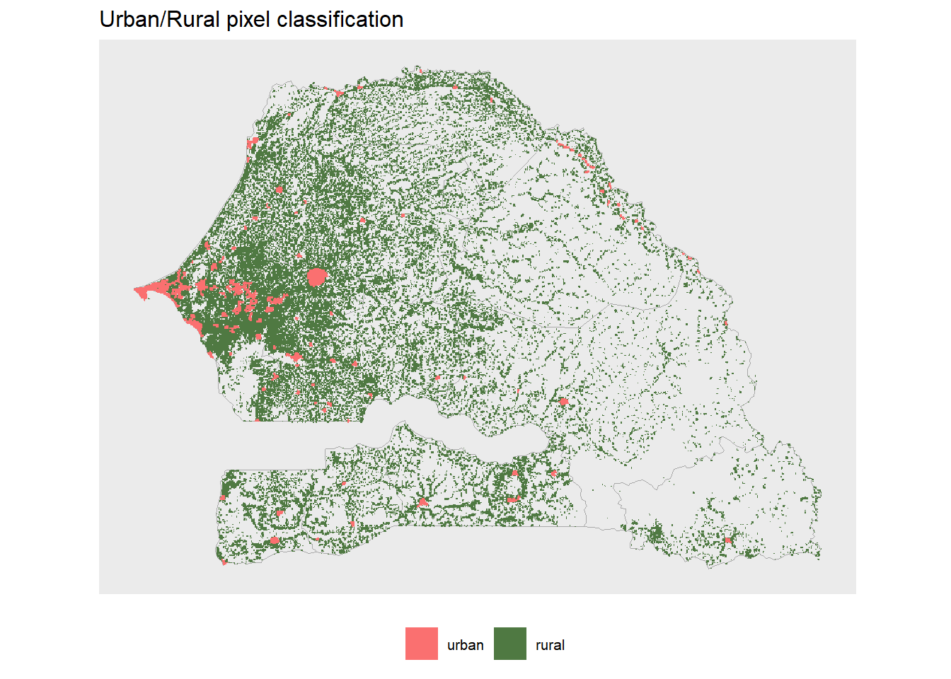
The function outputs a new raster which we have saved as an object in our R session called ur_population and ur_categories. This first is a raster is similar to population_raster input but all non-urban pixels are masked (i.e. NA). And the second a raster that classifies populated pixels as either urban or rural.
For performing this analysis for another country users can use the threshold values from the Eurostat manual, or if a national threshold is provided the user can select these. The Eurostat manual uses two definitions of urban at a level 1 classification.
Urban centre (high density cluster) - a cluster of contiguous grid cells of 1km² (using four-point contiguity, in other words, excluding diagonals. To perform 4 point contiguity in the
define_urban()function setdirections = 4in the function call) with a population density of at least 1,500 inhabitants per km² and collectively a minimum population of 50,000 inhabitants before gap-filling.Urban cluster (moderate-density cluster) — a cluster of contiguous grid cells of 1 km² (using eight-point contiguity, in other words, including diagonals) with a population density of at least 300 inhabitants per km² and a minimum population of 5,000 inhabitants.
Calculating the urban proportion of the population in a spatial area defined by an input shape file
To calcualte the proportion of the population in a spatial region that live in urban or rural areas we first need a shape file with defined boundaries e.g. administrative units or health facility catchment areas.
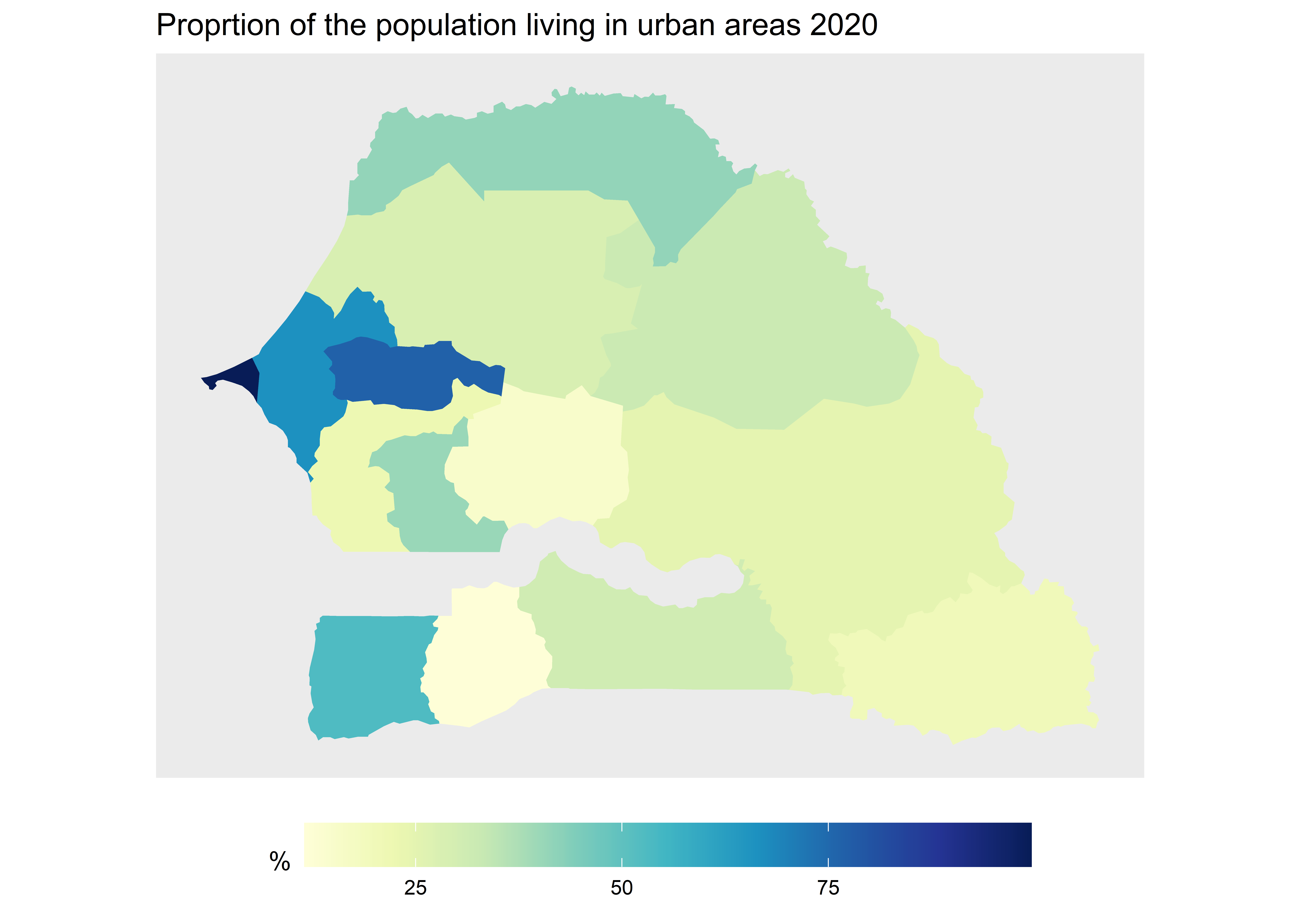
For this example we will use a shapefile of the 14 regions of Senegal.
# crop the raster to the shape file outline of senegal to ensure extents match
ur_population <- crop(ur_population, extent(shp))
ur_population <- mask(ur_population, shp)

# for ID-ing regions
sf_tibble <- tibble::as_tibble(sf::st_drop_geometry(shp))

# extract the full GRID3 population to admin-1 units
adm1_pop <-
    exactextractr::exact_extract(population_1km, shp, 'sum', progress = FALSE) %>%
    dplyr::bind_cols(sf_tibble) %>%
    dplyr::select(ADM1, total_pop = ...1)

# extract urban population to admin-1 units
adm1_urb_pop <-
    exactextractr::exact_extract(ur_population, shp, 'sum', progress = FALSE) %>%
    dplyr::bind_cols(sf_tibble) %>%
    dplyr::select(ADM1, urban_pop = ...1)

# join dataframes together and calculate proportion of the population in urban areas per admin-1 units
urb_pop_prop <-
  left_join(adm1_pop, adm1_urb_pop) %>%
  mutate(prop_ur = urban_pop / total_pop) %>%
  mutate(prop_ur = case_when(is.na(prop_ur) ~ 0, TRUE ~ prop_ur))

# plot the proportion of the population living in urban areas by admin-1 units
shp_pop <-
  shp %>%
  left_join(urb_pop_prop)

ggplot(shp_pop) +
  geom_sf(aes(fill=prop_ur*100), col=NA) +
  scale_fill_whitebox_c(palette= "deep") +
  theme_gray(10) +
  theme(axis.text = element_blank(),
        axis.ticks = element_blank(),
        panel.grid = element_blank(),
        legend.position="bottom",
        legend.key.width = unit(2, 'cm')) +
  labs(fill="%", title="Proprtion of the population living in urban areas 2020")
Classifying point locations based on urban rural pixel classifications
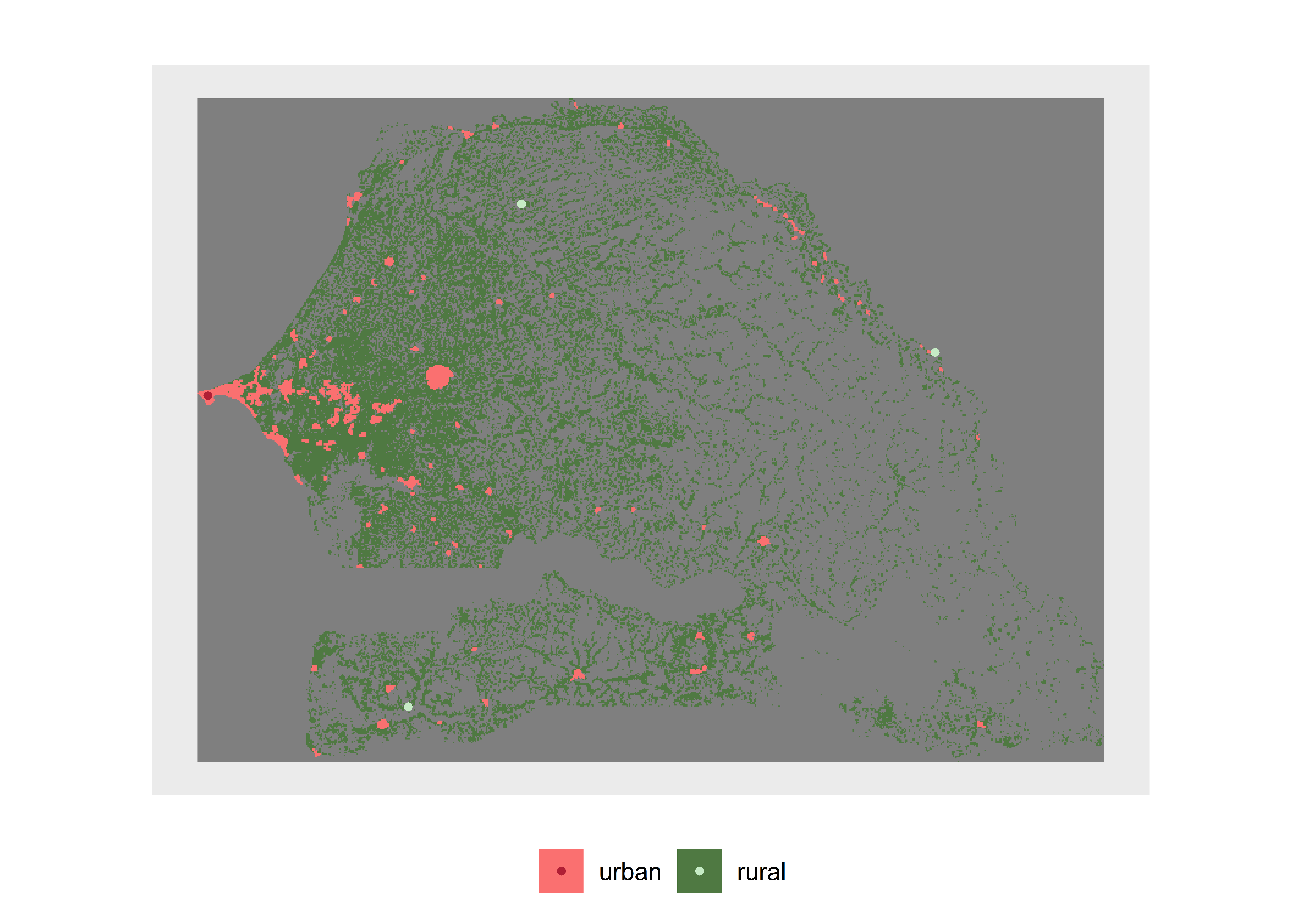
If geo-location or point data is avaliable, for example the co-ordinates of health facilities, hospitals, schools, pharmacies etc, then we can use the ur_categories raster output to classify these services and the communities they serve.
Here I create some example coordinates but users should upload their own coordinates of interest here. In this example we include a 2.5km buffer region around each point to account for potential heterogeneity that might be missed from taking just the point-level extraction.
# example coordinates
points <- data.frame(name = c("a", "b", "c", "d"),
                     latitude = c(14.72810, 15.01430, 15.99420, 12.67370),
                     longitude = c(-17.45910, -12.50030, -15.32010, -16.09250))

# transform to a spatial object
points   <- sf::st_as_sf(points,                                # first argument = data frame with coordinates
                          coords = c("longitude", "latitude"),  # name of columns, in quotation marks
                          crs = 4326)                           # coordinate reference system to make sense of the numbers

# include a 2.5km buffer region around point location
points_w_buffer <- terra::vect(points) %>% terra::buffer(width=2500)
Because we include a buffer region we will then take the mode of the extracted cell values for each of our locations. The following function calculates and returns the mode of the categorical extraction variables.
calculate_mode <- function(x) {
  uniqx <- unique(na.omit(x))
  uniqx[which.max(tabulate(match(x, uniqx)))]
}
Now we can run the extraction and examine the resulting classification.
# crop the raster to the shape file outline of senegal to ensure extents match
ur_categories <- crop(ur_categories, extent(shp))
ur_categories <- mask(ur_categories, shp)

# extraction
points_classification <-
  terra::extract(ur_categories, points_w_buffer) %>%
  dplyr::group_by(ID) %>%
  dplyr::summarise(dplyr::across(dplyr::everything(), list)) %>%
  tidyr::unnest(cols = c(urban_rural)) %>%
  dplyr::group_by(ID) %>%
  dplyr::summarize(classification = calculate_mode(urban_rural))

# as a spatial object
points_classification_sf <- bind_cols(points, points_classification)

# plot
ggplot() +
  geom_spatraster(data = ur_categories) +
  geom_sf(data = points_classification_sf, mapping=aes(col=classification), shape = 19,
          fill=NA, size=1)+
  theme_grey(12) +
  labs(title = "", fill=" ", col=" ") +
  scale_color_manual(values=c("#b01f35", "#C6EBC5"),
                     labels=c("urban", "rural"), breaks=c("urban", "rural")) +
  scale_fill_manual(values=c("#FA7070", "#4f7942"),
                    labels=c("urban", "rural"), breaks=c("urban", "rural")) +
  theme(axis.text = element_blank(),
        axis.ticks = element_blank(),
        panel.grid = element_blank(),
        legend.position="bottom")
Citation
@online{thompson2022,
  author = {Hayley Thompson},
  title = {Defining Urban Areas Based on Population Rasters},
  date = {2022-12-20},
  url = {https://github.com/PATH-Global-Health/MNTD-tech-docs/posts/urban-rural-pathtools},
  langid = {en}
}
