install.packages("dplyr")3 Topic 2: Data manipulation with *dplyr* and *tidyr*
4 Data Manipulation with dplyr and tidyr
4.1 The power of packages
One of the great things about using R are the thousands of available packages, which provide additional functions for many analytical tasks, such as data cleaning, statistical modelling, mapping, and much more. R packages are open-source, which means that they are free to use and maintained by the R community.
4.1.1 Installing and loading packages
Throughout the rest of this training we will use a set of R packages manipulating data and creating plots and maps. As we covered in Chapter 1, we first need to install the package on our computer using the install.packages() function. This only needs to be done one time (you probably already did this earlier).
Once the package has been installed, we can load it into our current R session using the library() function. Unlike installing, you will need to load the library each time you want to use it. This is because some libraries may have functions with the same names as other libraries or as our variables.
library(dplyr) For the next series of exercises, we will be using a group of packages which have been designed to work together to do common data science tasks. This group of packages is called the “Tidyverse”, because it is designed to work within the “tidy” data philosophy:
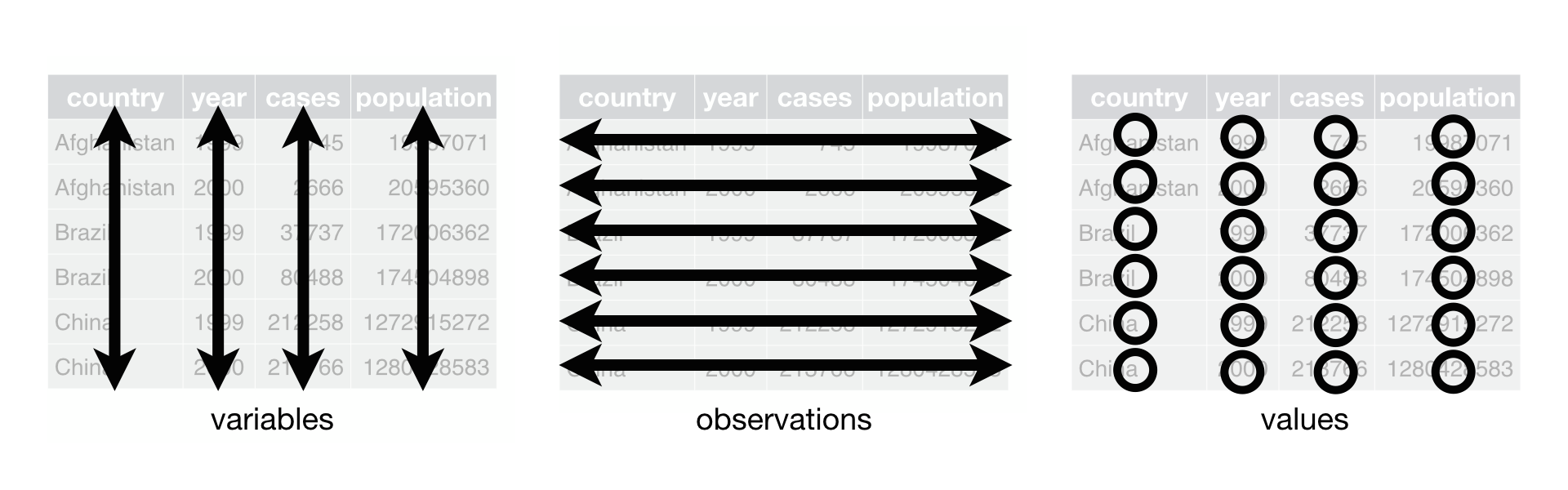
Some important qualities of this philosophy is that our data should have the following format:
- Each column should be a single variable with one data type.
- Each row should be a single observation.
- Each cell should be a single value contains one piece of information.
We can install all of these packages at once using install.package("tidyverse"). Remember that we only install the package once, so it is actually better to type this directly into the console instead of in our R script since it does not need to be repeated. Also be aware that this may take some time especially if internet quality is poor. After the package has finished installing it is ready to be loaded into our R session.
library(tidyverse)4.2 Reading data into R
Once the tidyverse package is loaded into our session we will have access to all of the functions in each of the Tidyverse packages. This includes packages for loading, manipulating, and plotting data. The function we will use is read_csv() to read in the district-level data we worked with previously. Note that this is similar but slightly different to the read.csv() function we used in our previous exercise.
case_data <- readRDS("data/district-cases-long-scrambled.rds")This is the same dataset we used in Chapter 1 (values scrambled to prevent unauthorized access to confidential data), only this time we called the object case_data instead of dat. It’s good practice to name your objects something short and meaningful, so that it’s easy to type and remember (this is especially useful when you have multiple data objects).
Also, in this file the data are organized in “long” format, whereas the file used in Chapter 1 was in “wide” format. We will discuss the difference between “long” and “wide” formatted data in this chapter, as well as how to change the shape of our data.
4.2.1 Inspecting data
Like in the previous exercise, we can use the head() and summary() functions to view aspects of the dataframe. We can also use the view() function to open the entire file in the R Studio Viewer, however view large files (millions of rows) can cause R Studio to crash. We can also install additional packages, such as skimr to get an even more detailed summary (run install.package("skimr") in your console).
head(case_data)
str(case_data)
summary(case_data)

# Using skimr package, remember to install first!
library(skimr)
skim(case_data)
Question 1: How many rows and columns are in case_data?
Question 2: What “type” of data are each column (character, vector, etc.)?
4.3 Data manipulation using *tidyverse*
In Chapter 1 we learned some built-in functions, or “base” functions, for simple data manipulations such as selecting a specific column or filter for only rows that match some criteria. In this lesson we will learn the *tidyverse* approach to these and additional common data manipulation tasks, using two packages called *dplyr* and *tidyr*. The *dplyr* package provides functions for the most common data manipulations jobs, and the *tidyr*package provides functions for reshaping or pivoting dataframes (similar to pivot tables in Microsoft Excel).
4.3.1 Selecting columns and filtering rows
To select a specific column from a dataframe, use the select() functions. The first argument will always be the dataframe object that you’re working with, followed by the name(s) of the column or columns you want to select.
# Select just one column (province)
select(case_data, province)
# Select multiple columns
select(case_data, district, data_type, count)
To select all the columns except certain ones, you can use a - in front of the column name.
# Select all but one column
select(case_data, -province)
# Removing multiple columns
select(case_data, -period, -province)
To choose specific rows based on some criteria, use filter(). Again, the first argument will be the dataframe, then the following argument will be the condition that we want use to subset the data.
filter(case_data, province == "Eastern")# A tibble: 2,294 × 5
# Rowwise:
period province district data_type count
<date> <chr> <chr> <chr> <dbl>
1 2018-01-01 Eastern Chadiza Clinical 89
2 2018-01-01 Eastern Chadiza Confirmed 3926
3 2018-01-01 Eastern Chadiza Tested 8261
4 2018-01-01 Eastern Chasefu Clinical 357
5 2018-01-01 Eastern Chasefu Confirmed 2599
6 2018-01-01 Eastern Chasefu Tested 9021
7 2018-01-01 Eastern Chipangali Confirmed 6330
8 2018-01-01 Eastern Chipangali Tested 21612
9 2018-01-01 Eastern Chipata Clinical 417
10 2018-01-01 Eastern Chipata Confirmed 4079
# ℹ 2,284 more rowsNotice here that just like in Chapter 1 use have to use a == sign for setting a condition. You read this as saying, “choose the rows in case_data where province is equal to”Eastern”. Also notice that the number of rows in the object has gone down from 18172 to 2294.
We can filter on multiple conditions at once using multiple arguments, using a , to state separate conditions.
filter(case_data, province == "Eastern", data_type == "Clinical")# A tibble: 379 × 5
# Rowwise:
period province district data_type count
<date> <chr> <chr> <chr> <dbl>
1 2018-01-01 Eastern Chadiza Clinical 89
2 2018-01-01 Eastern Chasefu Clinical 357
3 2018-01-01 Eastern Chipata Clinical 417
4 2018-01-01 Eastern Kasenengwa Clinical 331
5 2018-01-01 Eastern Katete Clinical 28
6 2018-01-01 Eastern Lumezi Clinical 19
7 2018-01-01 Eastern Lundazi Clinical 38
8 2018-01-01 Eastern Lusangazi Clinical 58
9 2018-01-01 Eastern Petauke Clinical 20
10 2018-01-01 Eastern Sinda Clinical 1
# ℹ 369 more rowsBy default, each of the conditions in filter() must be TRUE to remain in the subset, however there are special operators that allow for more complex conditional operations. The most common are the AND (&) and OR (|) operators. Here are some examples:
# Province is Easter AND data type is Clinical
filter(case_data, province == "Eastern" & data_type == "Clinical")

# Province is Eastern OR data type is Clinical
filter(case_data, province == "Eastern" | data_type == "Clinical")

# Province is Central OR Eastern, AND count is over 1,000
filter(case_data, province == "Central" | province == "Eastern", count > 1000)
Question 3: Why did we not use & in the third example?
Another useful operator is the MATCH operator (%in%), which will return TRUE if a value matches any value in a list of possible options.
# Keep rows where data type could be Clinical, Confirmed, or Tested
filter(case_data, data_type %in% c("Clinical", "Confirmed", "Tested"))
# A tibble: 13,062 × 5
# Rowwise:
period province district data_type count
<date> <chr> <chr> <chr> <dbl>
1 2018-01-01 Central Chibombo Clinical 26
2 2018-01-01 Central Chibombo Confirmed 1897
3 2018-01-01 Central Chibombo Tested 8215
4 2018-01-01 Central Chisamba Confirmed 2192
5 2018-01-01 Central Chisamba Tested 7772
6 2018-01-01 Central Chitambo Clinical 33
7 2018-01-01 Central Chitambo Confirmed 6011
8 2018-01-01 Central Chitambo Tested 3993
9 2018-01-01 Central Itezhi-tezhi Confirmed 890
10 2018-01-01 Central Itezhi-tezhi Tested 5007
# ℹ 13,052 more rows# Keep rows from a group of selected districts
study_districts <- c("Chadiza", "Chipata", "Katete", "Lumezi")
filter(case_data, district %in% study_districts)# A tibble: 649 × 5
# Rowwise:
period province district data_type count
<date> <chr> <chr> <chr> <dbl>
1 2018-01-01 Eastern Chadiza Clinical 89
2 2018-01-01 Eastern Chadiza Confirmed 3926
3 2018-01-01 Eastern Chadiza Tested 8261
4 2018-01-01 Eastern Chipata Clinical 417
5 2018-01-01 Eastern Chipata Confirmed 4079
6 2018-01-01 Eastern Chipata Tested 20550
7 2018-01-01 Eastern Katete Clinical 28
8 2018-01-01 Eastern Katete Confirmed 3124
9 2018-01-01 Eastern Katete Tested 18207
10 2018-01-01 Eastern Lumezi Clinical 19
# ℹ 639 more rowsQuestion 4: Can you show all of the “Tested” data in Western Province?
Question 5: Can you show all “Confirmed” that have a count over 2000?
Finally, the ! operator in R used for NOT or opposite conditions. The most common use cases are for using NOT EQUAL (!=) or does NOT MATCH operations.
# Keep all rows where province is NOT Lusaka
filter(case_data, province != "Lusaka")
# A tibble: 16,993 × 5
# Rowwise:
period province district data_type count
<date> <chr> <chr> <chr> <dbl>
1 2018-01-01 Central Chibombo Clinical 26
2 2018-01-01 Central Chibombo Confirmed 1897
3 2018-01-01 Central Chibombo Tested 8215
4 2018-01-01 Central Chisamba Confirmed 2192
5 2018-01-01 Central Chisamba Tested 7772
6 2018-01-01 Central Chitambo Clinical 33
7 2018-01-01 Central Chitambo Confirmed 6011
8 2018-01-01 Central Chitambo Tested 3993
9 2018-01-01 Central Itezhi-tezhi Confirmed 890
10 2018-01-01 Central Itezhi-tezhi Confirmed_Passive_CHW 897
# ℹ 16,983 more rows# Keep rows where data type does NOT match Clinical, Confirmed, or Tested
filter(case_data, !data_type %in% c("Clinical", "Confirmed", "Tested"))# A tibble: 5,110 × 5
# Rowwise:
period province district data_type count
<date> <chr> <chr> <chr> <dbl>
1 2018-01-01 Central Itezhi-tezhi Confirmed_Passive_CHW 897
2 2018-01-01 Central Itezhi-tezhi Tested_Passive_CHW 2708
3 2018-01-01 Central Mumbwa Confirmed_Passive_CHW 861
4 2018-01-01 Central Mumbwa Tested_Passive_CHW 3173
5 2018-01-01 Central Shibuyunji Confirmed_Passive_CHW 6
6 2018-01-01 Central Shibuyunji Tested_Passive_CHW 94
7 2018-01-01 Eastern Petauke Confirmed_Passive_CHW 0
8 2018-01-01 Eastern Petauke Tested_Passive_CHW 0
9 2018-01-01 Lusaka Chirundu Confirmed_Passive_CHW 55
10 2018-01-01 Lusaka Chirundu Tested_Passive_CHW 406
# ℹ 5,100 more rowsNote that for NOT EQUAL the ! operator comes right next to the = sign, but for the NOT MATCH condition the ! comes before the condition state. In the second case you can read that as, “do the opposite of this condition”.
Question 6a: Create a table for all malaria tests (health facility and CHW) in Western and Southern Province in 2020.
Question 6b: Create a table for all malaria tests (health facility and CHW) NOT in Western and Southern Province in 2020.
Question 7a: Create a table for all clinical and confirmed cases that are over 500.
Question 7b: Create a table for all data that are NOT clinical and confirmed cases that are over 500.
The types of conditional states that you can use depends on the type of column you want to base your filter()on. For example, filter(case_data, count > 1000) makes sense since the count column contains numeric data. However, filter(case_data, province > 1000) doesn’t make sense since the province column contains character data. The rule of thumb is that the value you use to set your condition should match the “type” of data in selected column.
In the next section, we see how to deal with a special case:
4.3.2 Working with dates using the *lubridate* package
In the “tidy” data approach to working with data each column is a specific type of data, each row is an observation, and each cell is an individual value which conveys a single piece of information. Our dataset matches this philosophy, except for the “period” values, which contain information on the year, month, and day of the observation.
We could create separate columns for the year, month, and day, but this may complicate our filtering. For instance, what happens if we want to filter for a study period that continues across over parts of adjacent months or year? Such a common task would require complex set of conditional statements to filter correctly.
The *lubridate* package provides a number of functions to make working with data much easier. This is not included in *tidyverse*, so we have to install and then load it into our session.
# install.packages(lubridate)
library(lubridate)
The ymd() function allows us to create a Date class object based on the string input for YEAR-MONTH-DAY:
# Vector of workshop days
workshop_days <- c("2021-11-15", "2021-11-16", "2021-11-17", "2021-11-18","2021-11-19")
class(workshop_days)
[1] "character"# Convert to a Date class
workshop_days <- ymd(workshop_days)
class(workshop_days)[1] "Date"Once you have a Date class object, *lubridate* provides many, many functions for working with date information. The primary functions we will use in this workshop are year() and month(), but there are many more in this *lubridate* cheatsheet.
year(workshop_days)[1] 2021 2021 2021 2021 2021month(workshop_days)[1] 11 11 11 11 11month(workshop_days, label = TRUE)[1] Nov Nov Nov Nov Nov
12 Levels: Jan < Feb < Mar < Apr < May < Jun < Jul < Aug < Sep < ... < DecThese functions can be used in filter().
filter(case_data, year(period) == 2020)# A tibble: 5,232 × 5
# Rowwise:
period province district data_type count
<date> <chr> <chr> <chr> <dbl>
1 2020-01-01 Central Chibombo Clinical 51
2 2020-01-01 Central Chibombo Confirmed 9473
3 2020-01-01 Central Chibombo Tested 17192
4 2020-01-01 Central Chisamba Confirmed 2885
5 2020-01-01 Central Chisamba Tested 5499
6 2020-01-01 Central Chitambo Clinical 1895
7 2020-01-01 Central Chitambo Confirmed 9929
8 2020-01-01 Central Chitambo Tested 12642
9 2020-01-01 Central Itezhi-tezhi Confirmed 1406
10 2020-01-01 Central Itezhi-tezhi Confirmed_Passive_CHW 1184
# ℹ 5,222 more rowsfilter(case_data, between(period, ymd("2019-01-01"), ymd("2019-06-30")))# A tibble: 2,394 × 5
# Rowwise:
period province district data_type count
<date> <chr> <chr> <chr> <dbl>
1 2019-01-01 Central Chibombo Clinical 347
2 2019-01-01 Central Chibombo Confirmed 3706
3 2019-01-01 Central Chibombo Tested 8116
4 2019-01-01 Central Chisamba Confirmed 2304
5 2019-01-01 Central Chisamba Tested 6975
6 2019-01-01 Central Chitambo Clinical 2
7 2019-01-01 Central Chitambo Confirmed 7328
8 2019-01-01 Central Chitambo Tested 8320
9 2019-01-01 Central Itezhi-tezhi Clinical 6
10 2019-01-01 Central Itezhi-tezhi Confirmed 833
# ℹ 2,384 more rowsQuestion 8: What were the reported total tests (HF and CHW) in Chadiza district each month during 2018?
Question 9: How many tests (HF and CHW) were conducted in April 2020 in Nchelenge district?
Question 10 (HARD): What were the monthly confirmed cases in Chadiza during the peak transmission season (December to May) each year?
4.3.3 Creating new columns with mutate()
Another common task is creating new columns based on values in existing columns. The *dplyr* function for this action is mutate().
Here is an example using the *lubridate* function from the section above to make a column for the year of observation:
mutate(case_data, year = year(period))# A tibble: 18,172 × 6
# Rowwise:
period province district data_type count year
<date> <chr> <chr> <chr> <dbl> <dbl>
1 2018-01-01 Central Chibombo Clinical 26 2018
2 2018-01-01 Central Chibombo Confirmed 1897 2018
3 2018-01-01 Central Chibombo Tested 8215 2018
4 2018-01-01 Central Chisamba Confirmed 2192 2018
5 2018-01-01 Central Chisamba Tested 7772 2018
6 2018-01-01 Central Chitambo Clinical 33 2018
7 2018-01-01 Central Chitambo Confirmed 6011 2018
8 2018-01-01 Central Chitambo Tested 3993 2018
9 2018-01-01 Central Itezhi-tezhi Confirmed 890 2018
10 2018-01-01 Central Itezhi-tezhi Confirmed_Passive_CHW 897 2018
# ℹ 18,162 more rowsFirst, state the name for the new column, then = followed by the function for the new value. You can create multiple new columns in a single mutate() call, using a , to separate each column.
mutate(case_data,
    year = year(period),
    month_num = month(period),
    month_name = month(period, label = TRUE))
# A tibble: 18,172 × 8
# Rowwise:
period province district data_type count year month_num month_name
<date> <chr> <chr> <chr> <dbl> <dbl> <dbl> <ord>
1 2018-01-01 Central Chibombo Clinical 26 2018 1 Jan
2 2018-01-01 Central Chibombo Confirmed 1897 2018 1 Jan
3 2018-01-01 Central Chibombo Tested 8215 2018 1 Jan
4 2018-01-01 Central Chisamba Confirmed 2192 2018 1 Jan
5 2018-01-01 Central Chisamba Tested 7772 2018 1 Jan
6 2018-01-01 Central Chitambo Clinical 33 2018 1 Jan
7 2018-01-01 Central Chitambo Confirmed 6011 2018 1 Jan
8 2018-01-01 Central Chitambo Tested 3993 2018 1 Jan
9 2018-01-01 Central Itezhi-tezhi Confirmed 890 2018 1 Jan
10 2018-01-01 Central Itezhi-tezhi Confirmed_… 897 2018 1 Jan
# ℹ 18,162 more rowsRemember that if you want to save any changes you will have to save the output into an object using the <- assignment operator.
case_data_dates <- mutate(case_data,
    year = year(period),
    month_num = month(period),
    month_name = month(period, label = TRUE))
In later sections we will see how to use mutate() to make calculations.
Question 11: Can you add a new variable (column) to the dataset that gives the quarter of the year?
Question 12: Can you add a new variable (column) to the dataset that gives just the last 2 digits of the year? i.e. 2021 becomes 21
4.4 Use Pipes to combine steps
What if you want to select and filter at the same time? There are three ways to do this: use intermediate steps, nested functions, or pipes.
For intermediate steps, we need to create a new intermediate object for the output of our first function, which will then be used as an input for the second function:
case_data_lusaka_confirmed <- filter(case_data, province == "Lusaka", data_type == "Confirmed")
case_data_lusaka_district_months <- select(case_data_lusaka_confirmed, district, period, count)
case_data_lusaka_district_months
# A tibble: 301 × 3
# Rowwise:
district period count
<chr> <date> <dbl>
1 Chilanga 2018-01-01 151
2 Chirundu 2018-01-01 198
3 Chongwe 2018-01-01 426
4 Kafue 2018-01-01 290
5 Luangwa 2018-01-01 776
6 Lusaka 2018-01-01 1248
7 Rufunsa 2018-01-01 2907
8 Chilanga 2018-02-01 165
9 Chirundu 2018-02-01 89
10 Chongwe 2018-02-01 467
# ℹ 291 more rowsThis approach is readable, but it can quickly clutter up your workspace and take up additional memory. And if you’re trying to use meaningful object names it can get tedious quickly.
You can also nest the functions (one function inside of the another).
case_data_lusaka_district_months <- select(
  filter(case_data, province == "Lusaka", data_type == "Confirmed"),
  district, period, count)
This doesn’t clutter the workshop or take up unnecessary memory, but it is difficult to read especially since R will interpret these steps from the inside out (first filter, then select).
The last option is to use pipes, a new addition to R. A pipe lets you take the output from one function and input it directly into the next function. By default, this will automatically go into the first argument of the new function. This is useful for stringing together multiple data cleaning steps while maintaining readability and keeping our environment clear. The *tidyverse* package includes a pipe function which looks like %>%. In RStudio, the shortcut for this pipe is Ctrl + Shift + M if you have a PC or Cmd + Shift + M if you have a Mac. You can adjust this shortcut under Tools >> Modify Keyboard Shortcuts…
Here’s an example of using a pipe for combine the filter and select from the previous example.
case_data %>%
  filter(province == "Lusaka", data_type == "Confirmed") %>%
  select(district, period, count)
# A tibble: 301 × 3
# Rowwise:
district period count
<chr> <date> <dbl>
1 Chilanga 2018-01-01 151
2 Chirundu 2018-01-01 198
3 Chongwe 2018-01-01 426
4 Kafue 2018-01-01 290
5 Luangwa 2018-01-01 776
6 Lusaka 2018-01-01 1248
7 Rufunsa 2018-01-01 2907
8 Chilanga 2018-02-01 165
9 Chirundu 2018-02-01 89
10 Chongwe 2018-02-01 467
# ℹ 291 more rowsIn this code, we used a pipe to send case_data into a filter() function and keep the rows for confirmed cases in Lusaka province, then used another pipe to send that output into a select() where we only kept the district, period, and count columns. We didn’t need to explicitly state the data object in the filter and select because data is always the first argument.
You may find it helpful to read the pipe like the word “then”. Take the case, then filter for Lusaka province and confirmed cases, then select the districts, periods, and counts. We can also save this into a new object.
lusaka_confirmed_cases <- case_data %>%
  filter(province == "Lusaka", data_type == "Confirmed") %>%
  select(district, period, count)
Question 13: Using pipes, create a table contain the confirmed cases in January 2019 for each district in Southern Province. The table should only have two columns (district and counts)
4.4.1 Grouping and summarizing data
Another common data manipulation tasks involve grouping data together and applying summary functions such as calculating means or totals. We can do some of these types of operations already. For instance, we can get the total number of clinical cases in Lusaka Province.
lusaka_clinical <- case_data %>%
  filter(data_type == "Clinical", province == "Lusaka")
sum(lusaka_clinical$count, na.rm = T)
[1] 68524But what if we want to get summaries for each province at once? We could repeat the steps above, separating each province, calculating the totals, and then grouping these summaries back together. In programming this concept is often referred to as the split-apply-combine paradigm. The key *dplyr* functions for these tasks are group_by() and summarize() (you can also use the “proper” summarise() spelling as well).
First, group_by() takes in a column that contains categorical data, then use summarize() to calculate new summary statistics.
case_data %>%
  filter(data_type == "Tested") %>%
  group_by(province) %>%
  summarise(mean_tested = mean(count, na.rm = TRUE))
# A tibble: 11 × 2
province mean_tested
<chr> <dbl>
1 Central 8199.
2 Copperbelt 15741.
3 Eastern 12389.
4 Luapula 9217.
5 Lusaka 5646.
6 Muchinga 8709.
7 Northern 7090.
8 Northwestern 10500.
9 Southern 1987.
10 Western 5524.
11 <NA> 1234.You can also group by more than one column, and output multiple columns within a single summarize() call.
case_data %>%
  filter(data_type == "Tested") %>%
  group_by(province, district, year(period)) %>%
  summarise(mean_tested_per_month = mean(count, na.rm = TRUE),
            total_tested_per_month = sum(count, na.rm = TRUE))
# A tibble: 466 × 5
# Groups: province, district [117]
province district `year(period)` mean_tested_per_month total_tested_per_month
<chr> <chr> <dbl> <dbl> <dbl>
1 Central Chibombo 2018 8442. 101301
2 Central Chibombo 2019 7309. 87711
3 Central Chibombo 2020 12910. 154926
4 Central Chibombo 2021 14252. 99763
5 Central Chisamba 2018 6959. 83511
6 Central Chisamba 2019 5204 62448
7 Central Chisamba 2020 5815. 69776
8 Central Chisamba 2021 5825. 40773
9 Central Chitambo 2018 4071. 48855
10 Central Chitambo 2019 5620. 67442
# ℹ 456 more rowscase_data %>%
filter(data_type == "Tested") %>%
group_by(province, district, year(period)) %>%
summarise(mean_tested_per_month = mean(count, na.rm = TRUE),
total_tested_per_month = sum(count, na.rm = TRUE))# A tibble: 466 × 5
# Groups: province, district [117]
province district `year(period)` mean_tested_per_month total_tested_per_month
<chr> <chr> <dbl> <dbl> <dbl>
1 Central Chibombo 2018 8442. 101301
2 Central Chibombo 2019 7309. 87711
3 Central Chibombo 2020 12910. 154926
4 Central Chibombo 2021 14252. 99763
5 Central Chisamba 2018 6959. 83511
6 Central Chisamba 2019 5204 62448
7 Central Chisamba 2020 5815. 69776
8 Central Chisamba 2021 5825. 40773
9 Central Chitambo 2018 4071. 48855
10 Central Chitambo 2019 5620. 67442
# ℹ 456 more rowsSometimes it is useful to rearrange the result of our summarized dataset, in which case we can use the arrange() function.
case_data %>%
  filter(data_type == "Tested",
         year(period) == 2019) %>%
  group_by(district, period) %>%
  summarise(total_tested_per_month = sum(count)) %>%
  arrange(total_tested_per_month)
# A tibble: 1,396 × 3
# Groups: district [117]
district period total_tested_per_month
<chr> <date> <dbl>
1 Mwandi 2019-10-01 45
2 Mwandi 2019-11-01 144
3 Mwandi 2019-01-01 267
4 Mwandi 2019-09-01 287
5 Mwandi 2019-12-01 292
6 Shang'ombo 2019-11-01 312
7 Pemba 2019-08-01 319
8 Shang'ombo 2019-07-01 348
9 Shang'ombo 2019-10-01 369
10 Mwandi 2019-06-01 389
# ℹ 1,386 more rowsBy default arranging with be in ascending order, you can use desc() to make the output descending.
case_data %>%
  filter(data_type == "Tested",
         year(period) == 2019) %>%
  group_by(district, period) %>%
  summarise(total_tested_per_month = sum(count)) %>%
  arrange(desc(total_tested_per_month))
# A tibble: 1,396 × 3
# Groups: district [117]
district period total_tested_per_month
<chr> <date> <dbl>
1 Kapiri-Mposhi 2019-03-01 53173
2 Kapiri-Mposhi 2019-04-01 45125
3 Petauke 2019-04-01 44856
4 Kitwe 2019-01-01 44378
5 Kapiri-Mposhi 2019-05-01 40387
6 Ndola 2019-04-01 39858
7 Kitwe 2019-02-01 39630
8 Chipangali 2019-04-01 39166
9 Solwezi 2019-12-01 38709
10 Kitwe 2019-03-01 37622
# ℹ 1,386 more rowsQuestion 14: What were the total number of confirmed cases in each province in 2019?
Question 15: What were the total number of cases (Clinical and Confirmed) in each month for all provinces for each year?
Question 16 (HARD): What were the total number of cases (Clinical and Confirmed) in the peak (dec - may) and the low (june - nov) transmission seasons for each district in Southern Province during the 2019/2020 transmission season (i.e. Dec 2019 - Nov 2020)?
4.5 Reshaping data with *tidyr*
So far we have covered a bunch of *dplyr* functions for manipulating data, most of which have changed the number of rows and/or columns in our dataframe. However, even though the columns, rows, and values have changed none of these have changed the “structure” of the dataframe. At the end of each function or piped function, the output always followed the conditions we discussed early:
- Each column should be a single variable with one data type.
- Each row should be a single observation.
- Each cell should be a single value contains one piece of information.
This is commonly referred to as “long” format data, and often this means that there are relatively more rows than columns. Typically it is best to work in “long” format data, especially in R, however there are instances when we may want to change the “shape” of our data into the “wide” format. In Microsoft Excel this would be called creating a Pivot Table.
The *tidyr* package provides functions for reshaping data, including creating “wide” format pivot tables. To illustrate, lets take a look at records for a single district at a single timepoint.
case_data %>%
  filter(district == "Chadiza", period == ymd("2020-01-01"))
# A tibble: 4 × 5
# Rowwise:
period province district data_type count
<date> <chr> <chr> <chr> <dbl>
1 2020-01-01 Eastern Chadiza Confirmed 3986
2 2020-01-01 Eastern Chadiza Confirmed_Passive_CHW 7321
3 2020-01-01 Eastern Chadiza Tested 8152
4 2020-01-01 Eastern Chadiza Tested_Passive_CHW 12297The resulting table has six rows, because there are six different types of records included. But what if we wanted to create a table where there is a separate column for each type of record? The pivot_wider() function will allow us to create this kind of “wide” format table. This function requires us to state the column which our column names will come from (names_from), and which column the values in the new columns will come from (values_from).
case_data %>%
  filter(district == "Chadiza", period == ymd("2020-01-01")) %>%
  pivot_wider(names_from = data_type, values_from = count)
# A tibble: 1 × 7
period province district Confirmed Confirmed_Passive_CHW Tested
<date> <chr> <chr> <dbl> <dbl> <dbl>
1 2020-01-01 Eastern Chadiza 3986 7321 8152
# ℹ 1 more variable: Tested_Passive_CHW <dbl>The resulting output just has one row, but new columns for each of the types of records. This “wide” format is often useful for creating summary tables.
The opposite function is called pivot_longer(), which will take in a “wide” format table and output a “long” format table. For pivot_longer() we need to state the column name for the “key” which provides the label, the column names for the values, and which columns we want to pivot on. Here is how we can convert the above example from “wide” format to “long” format.
wide_data <- case_data %>%
  filter(district == "Chadiza", period == ymd("2020-01-01")) %>%
  pivot_wider(names_from = data_type, values_from = count)


wide_data %>%
  pivot_longer(
    names_to = "data_type", values_to = "count",
    cols = c(Confirmed, Confirmed_Passive_CHW, Tested,
             Tested_Passive_CHW))
# A tibble: 4 × 5
period province district data_type count
<date> <chr> <chr> <chr> <dbl>
1 2020-01-01 Eastern Chadiza Confirmed 3986
2 2020-01-01 Eastern Chadiza Confirmed_Passive_CHW 7321
3 2020-01-01 Eastern Chadiza Tested 8152
4 2020-01-01 Eastern Chadiza Tested_Passive_CHW 12297Question 17: Create a table that contains the total number of confirmed cases each year for each province, then pivot wider to make it so the rows are the year and there is a column for each province.
Think of this as a multi-step process
1. Filter for confirmed cases
2. Work out which columns you are grouping by (i.e. what are we grouping over….think geography/time?)
3. Look at the output so far - what do we now want to sum over for our table?
4. Now we need to pivot wider - we want to make new columns - where do those names to come from (names_from)?, where will we find the values to populate the new cells (values_from)?
Question 17b: Can you make this table longer again, where we now have 3 columns - year, province and count
Question 18: Create a table that contains the total number of CHW tests for each district and each year in Luapula Province, now pivot wider to make each district its own column where year is now the row - start by writing out the steps 1 by 1 as above
4.6 Final Exercises
- For each province, calculate the total number of tests conducted by CHWs each year and present as a wide dataframe, where each column is a year and each row is a province and finally, order the dataframe such that the province with the most tests in 2020 is at the top
- For each district in Eastern Province, calculate the test positivity rate at health facilities and by CHWs in 2020 (Test positivity = confirmed cases / total tests)
Tips for Final Exercises 1. Start by filtering your data - what geographical region, year, and data types do we need?
2. Now we need to pivot wider - how can we now have data_type as our column names?
3. Now we need to group_by - what are we grouping by?
4. Almost there!! Now we need to sum up some columns - how can we do this?
5. Now to calculate TPR - let’s use the mutate function
6. Now let’s use the ‘select’ function to retrieve the columns we want
4.7 Function cheatsheet
*dplyr* functions
select(): subset columnsfilter(): subset rows on conditionmutate(): create new columnsgroup_by(): group data by one or more columnsummarise(): create summaries from dataframe (works within groups)arrange(): reorder dataframe based on ascending order (usedesc()to invert)
*tidyr* functions
pivot_wider(): go from “long” to “wide” formatpivot_longer(): go from “wide” to “long” format
*lubridate* functions
ymd(): convert class to date object based on “YYYY-MM-DD”year(): return the year from a date inputmonth(): return the month from a date inputquarter(): return the year quarter (1,2,3,4) from a date input