install.packages("dplyr")Data manipulation with dplyr and tidyr
The power of packages
One of the great things about using R are the thousands of available packages, which provide additional functions for many analytical tasks, such as data cleaning, statistical modelling, mapping, and much more. R packages are open-source, which means that they are free to use and maintained by the R community.
Installing and loading packages
Throughout the rest of the workshop we will use a set of R packages manipulating data and creating plots and maps. As we covered in the Day 1 lesson, we first need to install the package on our computer using the install.packages() function. This only needs to be done one time (you probably already did this earlier).
Once the package has been installed, we can load it into our current R session using the library() function. Unlike installing, you will need to load the library each time you want to use it. This is because some libraries may have functions with the same names as other libraries or as our variables.
library(dplyr) For the next series of exercises, we will be using a group of packages which have been designed to work together to do common data science tasks. This group of packages is called the “Tidyverse”, because it is designed to work within the “tidy” data philosophy:
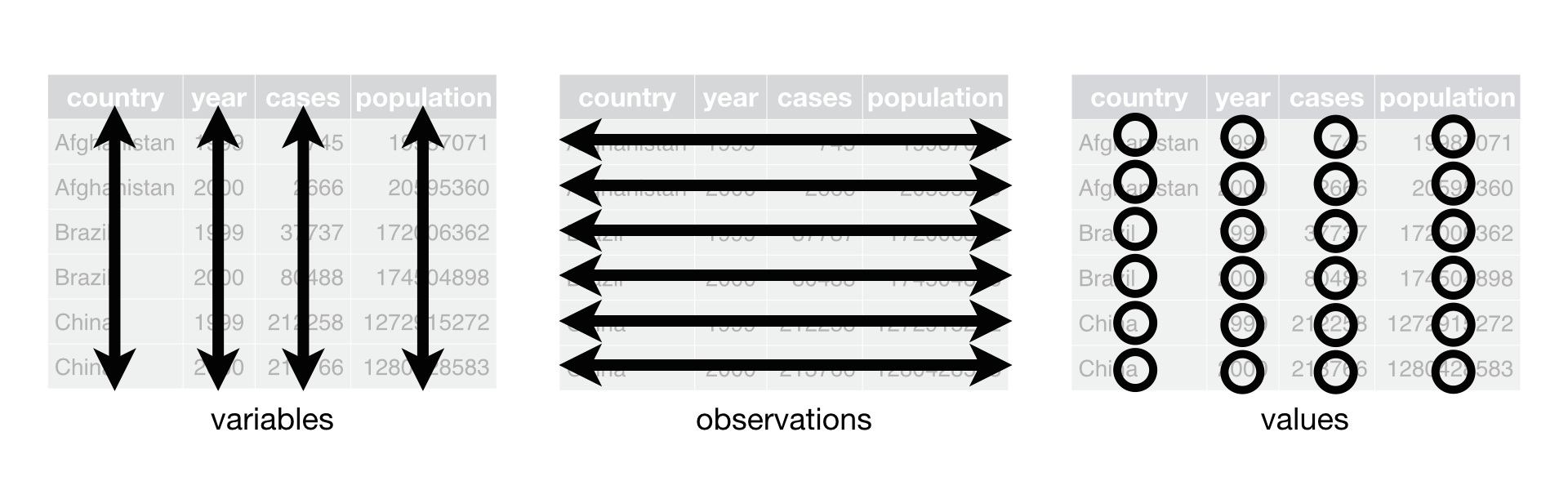
Some important qualities of this philosophy is that our data should have the following format:
- Each column should be a single variable with one data type.
- Each row should be a single observation.
- Each cell should be a single value contains one piece of information.
We can install all of these packages at once using install.package("tidyverse"). Remember that we only install the package once, so it is actually better to type this directly into the console instead of in our R script since it does not need to be repeated. Also be aware that this may take some time especially if internet quality is poor. After the package has finished installing it is ready to be loaded into our R session.
library(tidyverse)Warning: package 'ggplot2' was built under R version 4.3.3Warning: package 'tidyr' was built under R version 4.3.3Warning: package 'readr' was built under R version 4.3.3Reading data into R
Once the tidyverse package is loaded into our session we will have access to all of the functions in each of the Tidyverse packages. This includes packages for loading, manipulating, and plotting data. The function we will use is read_csv() to read in the woreda-level data we worked with previously. Note that this is similar but slightly different to the read.csv() function we used in our previous exercise.
case_data <- read_csv("data/training_case_data_long.csv")This is the same dataset we used in the Day 1 workshop, only this time we called the object case_data instead of dat. It’s good practice to name your objects something short and meaningful, so that it’s easy to type and remember (this is especially useful when you have multiple data objects).
Also, in this file the data are organized in “long” format, whereas the file used in Day 1 was in “wide” format. We will discuss the difference between “long” and “wide” formatted data in today’s material, as well as how to change the shape of our data.
Inspecting data
Like in the previous exercise, we can use the head() and summary() functions to view aspects of the dataframe. We can also use the view() function to open the entire file in the R Studio Viewer, however view large files (millions of rows) can cause R Studio to crash. We can also install additional packages, such as skimr to get an even more detailed summary (run install.package("skimr") in your console).
head(case_data)
str(case_data)
summary(case_data)

# Using skimr package, remember to install first!
library(skimr)
skim(case_data)
Question 1: How many rows and columns are in case_data?
Question 2: What “type” of data are each column (character, vector, etc.)?
Data manipulation using *tidyverse*
In the Day 1 workshop we learned some built-in functions, or “base” functions, for simple data manipulations such as selecting a specific column or filter for only rows that match some criteria. In this lesson we will learn the *tidyverse* approach to these and additional common data manipulation tasks, using two packages called *dplyr* and *tidyr*. The *dplyr* package provides functions for the most common data manipulations jobs, and the *tidyr*package provides functions for reshaping or pivoting dataframes (similar to pivot tables in Microsoft Excel).
Selecting columns and filtering rows
To select a specific column from a dataframe, use the select() function. The first argument will always be the dataframe object that you’re working with, followed by the name(s) of the column or columns you want to select.
# Select just one column (region)
select(case_data, region)
# Select multiple columns
select(case_data, woreda, data_type, count)
To select all the columns except certain ones, you can use a - in front of the column name.
# Select all but one column
select(case_data, -region)
# Removing multiple columns
select(case_data, -period, -region)
To choose specific rows based on some criteria, use filter(). Again, the first argument will be the dataframe, then the following argument will be the condition that we want use to subset the data.
filter(case_data, region == "Oromia")# A tibble: 32,064 × 7
region zone woreda year period data_type count
<chr> <chr> <chr> <dbl> <date> <chr> <dbl>
1 Oromia Horo Gudru Wellega Ababo 2018 2018-01-01 confirmed NA
2 Oromia Horo Gudru Wellega Ababo 2018 2018-02-01 confirmed NA
3 Oromia Horo Gudru Wellega Ababo 2018 2018-03-01 confirmed NA
4 Oromia Horo Gudru Wellega Ababo 2018 2018-04-01 confirmed NA
5 Oromia Horo Gudru Wellega Ababo 2018 2018-05-01 confirmed NA
6 Oromia Horo Gudru Wellega Ababo 2018 2018-06-01 confirmed NA
7 Oromia Horo Gudru Wellega Ababo 2018 2018-07-01 confirmed 16
8 Oromia Horo Gudru Wellega Ababo 2018 2018-08-01 confirmed 83
9 Oromia Horo Gudru Wellega Ababo 2018 2018-09-01 confirmed 35
10 Oromia Horo Gudru Wellega Ababo 2018 2018-10-01 confirmed 167
# ℹ 32,054 more rowsNotice here that just like in Day 1 use have to use a == sign for setting a condition. You can read this as saying, “choose the rows in case_data where region is equal to”Oromia”. Also notice that the number of rows in the object has gone down from 94176 to 32064.
We can filter on multiple conditions at once using multiple arguments, using a , to state separate conditions.
filter(case_data, region == "Oromia", data_type == "presumed")# A tibble: 16,032 × 7
region zone woreda year period data_type count
<chr> <chr> <chr> <dbl> <date> <chr> <dbl>
1 Oromia Horo Gudru Wellega Ababo 2018 2018-01-01 presumed NA
2 Oromia Horo Gudru Wellega Ababo 2018 2018-02-01 presumed NA
3 Oromia Horo Gudru Wellega Ababo 2018 2018-03-01 presumed NA
4 Oromia Horo Gudru Wellega Ababo 2018 2018-04-01 presumed NA
5 Oromia Horo Gudru Wellega Ababo 2018 2018-05-01 presumed NA
6 Oromia Horo Gudru Wellega Ababo 2018 2018-06-01 presumed NA
7 Oromia Horo Gudru Wellega Ababo 2018 2018-07-01 presumed NA
8 Oromia Horo Gudru Wellega Ababo 2018 2018-08-01 presumed NA
9 Oromia Horo Gudru Wellega Ababo 2018 2018-09-01 presumed NA
10 Oromia Horo Gudru Wellega Ababo 2018 2018-10-01 presumed NA
# ℹ 16,022 more rowsBy default, each of the conditions in filter() must be TRUE to remain in the subset, however there are special operators that allow for more complex conditional operations. The most common are the AND (&) and OR (|) operators. Here are some examples:
# region is Easter AND data type is presumed
filter(case_data, region == "Oromia" & data_type == "presumed")

# region is Oromia OR data type is presumed
filter(case_data, region == "Oromia" | data_type == "presumed")

# region is Afar OR Oromia, AND count is over 1,000
filter(case_data, region == "Afar" | region == "Oromia", count > 1000)
Question 3: Why did we not use & in the third example?
Another useful operator is the MATCH operator (%in%), which will return TRUE if a value matches any value in a list of possible options.
# Keep rows where data type could be presumed or confirmed
filter(case_data, data_type %in% c("presumed", "confirmed"))
# A tibble: 94,176 × 7
region zone woreda year period data_type count
<chr> <chr> <chr> <dbl> <date> <chr> <dbl>
1 Somali Shabelle Aba-Korow 2018 2018-01-01 confirmed NA
2 Somali Shabelle Aba-Korow 2018 2018-02-01 confirmed NA
3 Somali Shabelle Aba-Korow 2018 2018-03-01 confirmed NA
4 Somali Shabelle Aba-Korow 2018 2018-04-01 confirmed NA
5 Somali Shabelle Aba-Korow 2018 2018-05-01 confirmed NA
6 Somali Shabelle Aba-Korow 2018 2018-06-01 confirmed NA
7 Somali Shabelle Aba-Korow 2018 2018-07-01 confirmed 21
8 Somali Shabelle Aba-Korow 2018 2018-08-01 confirmed 13
9 Somali Shabelle Aba-Korow 2018 2018-09-01 confirmed 37
10 Somali Shabelle Aba-Korow 2018 2018-10-01 confirmed 20
# ℹ 94,166 more rows# Keep rows from a group of selected woredas
study_woredas <- c("Adama Town", "Liban Jawi", "Mieso", "Wondo")
filter(case_data, woreda %in% study_woredas)# A tibble: 384 × 7
region zone woreda year period data_type count
<chr> <chr> <chr> <dbl> <date> <chr> <dbl>
1 Oromia East Shewa Adama Town 2018 2018-01-01 confirmed NA
2 Oromia East Shewa Adama Town 2018 2018-02-01 confirmed NA
3 Oromia East Shewa Adama Town 2018 2018-03-01 confirmed NA
4 Oromia East Shewa Adama Town 2018 2018-04-01 confirmed NA
5 Oromia East Shewa Adama Town 2018 2018-05-01 confirmed NA
6 Oromia East Shewa Adama Town 2018 2018-06-01 confirmed NA
7 Oromia East Shewa Adama Town 2018 2018-07-01 confirmed NA
8 Oromia East Shewa Adama Town 2018 2018-08-01 confirmed NA
9 Oromia East Shewa Adama Town 2018 2018-09-01 confirmed NA
10 Oromia East Shewa Adama Town 2018 2018-10-01 confirmed NA
# ℹ 374 more rowsQuestion 4: Can you show all of the “presumed” data in the Somali region?
Question 5: Can you show all “confirmed” that have a count over 2000?
Finally, the ! operator in R used for NOT or opposite conditions. The most common use cases are for using NOT EQUAL (!=) or does NOT MATCH operations.
# Keep all rows where region is NOT oromia
filter(case_data, region != "Addis Ababa")
# A tibble: 93,216 × 7
region zone woreda year period data_type count
<chr> <chr> <chr> <dbl> <date> <chr> <dbl>
1 Somali Shabelle Aba-Korow 2018 2018-01-01 confirmed NA
2 Somali Shabelle Aba-Korow 2018 2018-02-01 confirmed NA
3 Somali Shabelle Aba-Korow 2018 2018-03-01 confirmed NA
4 Somali Shabelle Aba-Korow 2018 2018-04-01 confirmed NA
5 Somali Shabelle Aba-Korow 2018 2018-05-01 confirmed NA
6 Somali Shabelle Aba-Korow 2018 2018-06-01 confirmed NA
7 Somali Shabelle Aba-Korow 2018 2018-07-01 confirmed 21
8 Somali Shabelle Aba-Korow 2018 2018-08-01 confirmed 13
9 Somali Shabelle Aba-Korow 2018 2018-09-01 confirmed 37
10 Somali Shabelle Aba-Korow 2018 2018-10-01 confirmed 20
# ℹ 93,206 more rowsNote that for NOT EQUAL the ! operator comes next to the = sign, but for the NOT MATCH condition the ! comes before the condition state. In the second case you can read that as, “do the opposite of this condition”.
Question 6a: Create a table for all confirmed malaria cases in Amhara and Harari regions in 2020.
Question 6b: Create a table for all presumed malaria cases NOT in Amhara and Harari regions in 2020.
Question 7a: Create a table for all presumed and confirmed cases that are over 500.
Question 7b: Create a table for all data that are NOT presumed and that are over 500.
The types of conditional states that you can use depends on the type of column you want to base your filter()on. For example, filter(case_data, count > 1000) makes sense since the count column contains numeric data. However, filter(case_data, region > 1000) doesn’t make sense since the region column contains character data. The rule of thumb is that the value you use to set your condition should match the “type” of data in selected column.
In the next section, we see how to deal with a special case:
Working with dates using the *lubridate* package
In the “tidy” data approach to working with data each column is a specific type of data, each row is an observation, and each cell is an individual value which conveys a single piece of information. Our dataset matches this philosophy, except for the “period” values, which contain information on the year, month, and day of the observation.
We could create separate columns for the year, month, and day, but this may complicate our filtering. For instance, what happens if we want to filter for a study period that continues across over parts of adjacent months or year? Such a common task would require complex set of conditional statements to filter correctly.
The *lubridate* package provides a number of functions to make working with data much easier. This is not included in *tidyverse*, so we have to install and then load it into our session.
# install.packages(lubridate)
library(lubridate)
The ymd() function allows us to create a Date class object based on the string input for YEAR-MONTH-DAY:
# Vector of workshop days
workshop_days <- c("2023-09-04", "2023-09-05", "2023-09-06", "2023-09-07","2023-09-08")
class(workshop_days)
[1] "character"# Convert to a Date class
workshop_days <- ymd(workshop_days)
class(workshop_days)[1] "Date"Once you have a Date class object, *lubridate* provides many, many functions for working with date information. The primary functions we will use in this workshop are year() and month(), but there are many more in this *lubridate* cheatsheet.
year(workshop_days)[1] 2023 2023 2023 2023 2023month(workshop_days)[1] 9 9 9 9 9month(workshop_days, label = TRUE)[1] Sep Sep Sep Sep Sep
12 Levels: Jan < Feb < Mar < Apr < May < Jun < Jul < Aug < Sep < ... < DecThese functions can be used in filter().
filter(case_data, year(period) == 2020)# A tibble: 23,544 × 7
region zone woreda year period data_type count
<chr> <chr> <chr> <dbl> <date> <chr> <dbl>
1 Somali Shabelle Aba-Korow 2020 2020-01-01 confirmed NA
2 Somali Shabelle Aba-Korow 2020 2020-02-01 confirmed NA
3 Somali Shabelle Aba-Korow 2020 2020-03-01 confirmed NA
4 Somali Shabelle Aba-Korow 2020 2020-04-01 confirmed NA
5 Somali Shabelle Aba-Korow 2020 2020-05-01 confirmed NA
6 Somali Shabelle Aba-Korow 2020 2020-06-01 confirmed NA
7 Somali Shabelle Aba-Korow 2020 2020-07-01 confirmed NA
8 Somali Shabelle Aba-Korow 2020 2020-08-01 confirmed NA
9 Somali Shabelle Aba-Korow 2020 2020-09-01 confirmed 15
10 Somali Shabelle Aba-Korow 2020 2020-10-01 confirmed NA
# ℹ 23,534 more rowsfilter(case_data, between(period, ymd("2019-01-01"), ymd("2019-06-30")))# A tibble: 11,772 × 7
region zone woreda year period data_type count
<chr> <chr> <chr> <dbl> <date> <chr> <dbl>
1 Somali Shabelle Aba-Korow 2019 2019-01-01 confirmed NA
2 Somali Shabelle Aba-Korow 2019 2019-02-01 confirmed NA
3 Somali Shabelle Aba-Korow 2019 2019-03-01 confirmed NA
4 Somali Shabelle Aba-Korow 2019 2019-04-01 confirmed NA
5 Somali Shabelle Aba-Korow 2019 2019-05-01 confirmed NA
6 Somali Shabelle Aba-Korow 2019 2019-06-01 confirmed NA
7 Afar Zone 2 (Kilbet Rasu) Aba 'Ala 2019 2019-01-01 confirmed 55
8 Afar Zone 2 (Kilbet Rasu) Aba 'Ala 2019 2019-02-01 confirmed 26
9 Afar Zone 2 (Kilbet Rasu) Aba 'Ala 2019 2019-03-01 confirmed 9
10 Afar Zone 2 (Kilbet Rasu) Aba 'Ala 2019 2019-04-01 confirmed 25
# ℹ 11,762 more rowsQuestion 8: What were the reported total cases (presumed and confirmed) in Bambasi woreda each month during 2018?
Question 9: How many cases (presumed and confirmed) were reported in April 2020 in Gudetu Kondole woreda?
Question 10 (HARD): What were the monthly confirmed cases in Bambasi during the peak transmission season (~September-December) each year?
Creating new columns with mutate()
Another common task is creating new columns based on values in existing columns. The *dplyr* function for this action is mutate().
Here is an example using the *lubridate* function from the section above to make a column for the month of observation:
mutate(case_data, month = month(period))# A tibble: 94,176 × 8
region zone woreda year period data_type count month
<chr> <chr> <chr> <dbl> <date> <chr> <dbl> <dbl>
1 Somali Shabelle Aba-Korow 2018 2018-01-01 confirmed NA 1
2 Somali Shabelle Aba-Korow 2018 2018-02-01 confirmed NA 2
3 Somali Shabelle Aba-Korow 2018 2018-03-01 confirmed NA 3
4 Somali Shabelle Aba-Korow 2018 2018-04-01 confirmed NA 4
5 Somali Shabelle Aba-Korow 2018 2018-05-01 confirmed NA 5
6 Somali Shabelle Aba-Korow 2018 2018-06-01 confirmed NA 6
7 Somali Shabelle Aba-Korow 2018 2018-07-01 confirmed 21 7
8 Somali Shabelle Aba-Korow 2018 2018-08-01 confirmed 13 8
9 Somali Shabelle Aba-Korow 2018 2018-09-01 confirmed 37 9
10 Somali Shabelle Aba-Korow 2018 2018-10-01 confirmed 20 10
# ℹ 94,166 more rowsFirst, state the name for the new column, then = followed by the function for the new value. You can create multiple new columns in a single mutate() call, using a , to separate each column.
mutate(case_data,
    month_num = month(period),
    month_name = month(period, label = TRUE))
# A tibble: 94,176 × 9
region zone woreda year period data_type count month_num month_name
<chr> <chr> <chr> <dbl> <date> <chr> <dbl> <dbl> <ord>
1 Somali Shabelle Aba-Ko… 2018 2018-01-01 confirmed NA 1 Jan
2 Somali Shabelle Aba-Ko… 2018 2018-02-01 confirmed NA 2 Feb
3 Somali Shabelle Aba-Ko… 2018 2018-03-01 confirmed NA 3 Mar
4 Somali Shabelle Aba-Ko… 2018 2018-04-01 confirmed NA 4 Apr
5 Somali Shabelle Aba-Ko… 2018 2018-05-01 confirmed NA 5 May
6 Somali Shabelle Aba-Ko… 2018 2018-06-01 confirmed NA 6 Jun
7 Somali Shabelle Aba-Ko… 2018 2018-07-01 confirmed 21 7 Jul
8 Somali Shabelle Aba-Ko… 2018 2018-08-01 confirmed 13 8 Aug
9 Somali Shabelle Aba-Ko… 2018 2018-09-01 confirmed 37 9 Sep
10 Somali Shabelle Aba-Ko… 2018 2018-10-01 confirmed 20 10 Oct
# ℹ 94,166 more rowsRemember that if you want to save any changes you will have to save the output into an object using the <- assignment operator. Otherwise then will not be updated in your variable.
case_data_dates <- mutate(case_data,
    month_num = month(period),
    month_name = month(period, label = TRUE))
In later sections we will see how to use mutate() to make calculations.
Question 11: Can you add a new variable (column) to the dataset that gives the quarter of the year?
Question 12: Can you add a new variable (column) to the dataset that gives just the last 2 digits of the year? i.e. 2021 becomes 21
Use Pipes to combine steps
What if you want to select and filter at the same time? There are three ways to do this: use intermediate steps, nested functions, or pipes.
For intermediate steps, we need to create a new intermediate object for the output of our first function, which will then be used as an input for the second function:
case_data_oromia_confirmed <- filter(case_data, region == "Oromia", data_type == "confirmed")
case_data_oromia_woreda_months <- select(case_data_oromia_confirmed, woreda, period, count)
case_data_oromia_woreda_months
# A tibble: 16,032 × 3
woreda period count
<chr> <date> <dbl>
1 Ababo 2018-01-01 NA
2 Ababo 2018-02-01 NA
3 Ababo 2018-03-01 NA
4 Ababo 2018-04-01 NA
5 Ababo 2018-05-01 NA
6 Ababo 2018-06-01 NA
7 Ababo 2018-07-01 16
8 Ababo 2018-08-01 83
9 Ababo 2018-09-01 35
10 Ababo 2018-10-01 167
# ℹ 16,022 more rowsThis approach is readable, but it can quickly clutter up your workspace and take up additional memory. And if you’re trying to use meaningful object names it can get tedious quickly.
You can also nest the functions (one function inside of the another).
case_data_oromia_woreda_months <- select(
  filter(case_data, region == "Oromia", data_type == "confirmed"),
  woreda, period, count)
This doesn’t clutter the workshop or take up unnecessary memory, but it is difficult to read especially since R will interpret these steps from the inside out (first filter, then select).
The last option is to use pipes, a new addition to R. A pipe lets you take the output from one function and input it directly into the next function. By default, this will automatically go into the first argument of the new function. This is useful for stringing together multiple data cleaning steps while maintaining readability and keeping our environment clear. The *tidyverse* package includes a pipe function which looks like %>%. In RStudio, the shortcut for this pipe is Ctrl + Shift + M if you have a PC or Cmd + Shift + M if you have a Mac. You can adjust this shortcut under Tools >> Modify Keyboard Shortcuts…
Here’s an example of using a pipe for combine the filter and select from the previous example.
case_data %>%
  filter(region == "Oromia", data_type == "confirmed") %>%
  select(woreda, period, count)
# A tibble: 16,032 × 3
woreda period count
<chr> <date> <dbl>
1 Ababo 2018-01-01 NA
2 Ababo 2018-02-01 NA
3 Ababo 2018-03-01 NA
4 Ababo 2018-04-01 NA
5 Ababo 2018-05-01 NA
6 Ababo 2018-06-01 NA
7 Ababo 2018-07-01 16
8 Ababo 2018-08-01 83
9 Ababo 2018-09-01 35
10 Ababo 2018-10-01 167
# ℹ 16,022 more rowsIn this code, we used a pipe to send case_data into a filter() function and keep the rows for confirmed cases in Oromia region, then used another pipe to send that output into a select() where we only kept the woreda, period, and count columns. We didn’t need to explicitly state the data object in the filter and select because data is always the first argument.
You may find it helpful to read the pipe like the word “then”. Take the case, then filter for Oromia region and confirmed cases, then select the woredas, periods, and counts. We can also save this into a new object.
oromia_confirmed_cases <- case_data %>%
  filter(region == "Oromia", data_type == "confirmed") %>%
  select(woreda, period, count)
Question 13: Using pipes, create a table contain the confirmed cases in January 2019 for each woreda in Oromia region. The table should only have two columns (woreda and count)
Grouping and summarizing data
Another common data manipulation task involves grouping data together and applying summary functions such as calculating means or totals. We can do some of these types of operations already. For instance, we can get the total number of presumed cases in Oromia region.
oromia_presumed <- case_data %>%
  filter(data_type == "presumed", region == "Oromia")
sum(oromia_presumed$count, na.rm = T)
[1] 58132But what if we want to get summaries for each region at once? We could repeat the steps above, separating each region, calculating the totals, and then grouping these summaries back together. In programming this concept is often referred to as the split-apply-combine paradigm. The key *dplyr* functions for these tasks are group_by() and summarize() (you can also use the “proper” summarise() spelling as well).
First, group_by() takes in a column that contains categorical data, then use summarize() to calculate new summary statistics.
case_data %>%
  filter(data_type == "presumed") %>%
  group_by(region) %>%
  summarise(mean_presumed = mean(count, na.rm = TRUE))
# A tibble: 11 × 2
region mean_presumed
<chr> <dbl>
1 Addis Ababa 13.2
2 Afar 52.2
3 Amhara 24.9
4 Benishangul Gumz 45.5
5 Dire Dawa 6.54
6 Gambela 70.3
7 Harari 12.2
8 Oromia 16.9
9 SNNP 29.6
10 Somali 54.8
11 Tigray 56.6 You can also group by more than one column, and output multiple columns within a single summarize() call.
case_data %>%
  filter(data_type == "presumed") %>%
  group_by(region, woreda, year) %>%
  summarise(mean_presumed_per_month = mean(count, na.rm = TRUE),
            total_presumed_per_month = sum(count, na.rm = TRUE))
# A tibble: 3,924 × 5
# Groups: region, woreda [981]
region woreda year mean_presumed_per_mo…¹ total_presumed_per_m…²
<chr> <chr> <dbl> <dbl> <dbl>
1 Addis Ababa Addis Ketema 2018 19.3 212
2 Addis Ababa Addis Ketema 2019 66.6 666
3 Addis Ababa Addis Ketema 2020 15.8 158
4 Addis Ababa Addis Ketema 2021 2.67 24
5 Addis Ababa Akaki - Kalit 2018 24.7 272
6 Addis Ababa Akaki - Kalit 2019 66.3 729
7 Addis Ababa Akaki - Kalit 2020 30.1 331
8 Addis Ababa Akaki - Kalit 2021 27.8 278
9 Addis Ababa Arada 2018 1.75 14
10 Addis Ababa Arada 2019 2.14 15
# ℹ 3,914 more rows
# ℹ abbreviated names: ¹mean_presumed_per_month, ²total_presumed_per_monthcase_data %>%
filter(data_type == "presumed") %>%
group_by(region, woreda, year) %>%
summarise(mean_presumed_per_month = mean(count, na.rm = TRUE),
total_presumed_per_month = sum(count, na.rm = TRUE))# A tibble: 3,924 × 5
# Groups: region, woreda [981]
region woreda year mean_presumed_per_mo…¹ total_presumed_per_m…²
<chr> <chr> <dbl> <dbl> <dbl>
1 Addis Ababa Addis Ketema 2018 19.3 212
2 Addis Ababa Addis Ketema 2019 66.6 666
3 Addis Ababa Addis Ketema 2020 15.8 158
4 Addis Ababa Addis Ketema 2021 2.67 24
5 Addis Ababa Akaki - Kalit 2018 24.7 272
6 Addis Ababa Akaki - Kalit 2019 66.3 729
7 Addis Ababa Akaki - Kalit 2020 30.1 331
8 Addis Ababa Akaki - Kalit 2021 27.8 278
9 Addis Ababa Arada 2018 1.75 14
10 Addis Ababa Arada 2019 2.14 15
# ℹ 3,914 more rows
# ℹ abbreviated names: ¹mean_presumed_per_month, ²total_presumed_per_monthSometimes it is useful to rearrange the result of our summarized dataset, in which case we can use the arrange() function.
case_data %>%
  filter(data_type == "presumed",
         year(period) == 2019) %>%
  group_by(woreda, period) %>%
  summarise(total_presumed_per_month = sum(count)) %>%
  arrange(total_presumed_per_month)
# A tibble: 11,760 × 3
# Groups: woreda [980]
woreda period total_presumed_per_month
<chr> <date> <dbl>
1 Ada'a 2019-10-01 1
2 Ada'a 2019-11-01 1
3 Addi Arekay 2019-09-01 1
4 Addis Ketema 2019-09-01 1
5 Adhaki 2019-10-01 1
6 Adigrat Town 2019-01-01 1
7 Adola Town 2019-04-01 1
8 Adola Town 2019-08-01 1
9 Adola Town 2019-09-01 1
10 Adola Town 2019-11-01 1
# ℹ 11,750 more rowsBy default arranging with be in ascending order, you can use desc() to make the output descending.
case_data %>%
  filter(data_type == "presumed",
         year(period) == 2019) %>%
  group_by(woreda, period) %>%
  summarise(total_presumed_per_month = sum(count)) %>%
  arrange(desc(total_presumed_per_month))
# A tibble: 11,760 × 3
# Groups: woreda [980]
woreda period total_presumed_per_month
<chr> <date> <dbl>
1 Goro Baqaqsa 2019-09-01 838
2 Tselemti 2019-11-01 801
3 Tsegede (Tigray) 2019-10-01 628
4 Tsegede (Tigray) 2019-11-01 620
5 Mirab Armacho 2019-10-01 616
6 Metema 2019-10-01 606
7 Tselemti 2019-12-01 575
8 Jawi 2019-10-01 557
9 Chwaka 2019-11-01 551
10 Bambasi 2019-10-01 550
# ℹ 11,750 more rowsQuestion 14: What were the total number of confirmed cases in each region in 2019?
Question 15: What were the total number of cases (presumed and confirmed) in each month for all regions for each year?
Question 16 (HARD): What were the total number of cases (presumed and confirmed) in the peak (September - December) and the low (January - April) transmission seasons for each woreda in Somali region during 2020?
Reshaping data with *tidyr*
So far we have covered a bunch of *dplyr* functions for manipulating data, most of which have changed the number of rows and/or columns in our dataframe. However, even though the columns, rows, and values have changed none of these have changed the “structure” of the dataframe. At the end of each function or piped function, the output always followed the conditions we discussed early:
- Each column should be a single variable with one data type.
- Each row should be a single observation.
- Each cell should be a single value contains one piece of information.
This is commonly referred to as “long” format data, and often this means that there are relatively more rows than columns. Typically it is best to work in “long” format data, especially in R, however there are instances when we may want to change the “shape” of our data into the “wide” format. In Microsoft Excel this would be called creating a Pivot Table.
The *tidyr* package provides functions for reshaping data, including creating “wide” format pivot tables. To illustrate, lets take a look at records for a single woreda at a single timepoint.
case_data %>%
  filter(woreda == "Awabel", period == ymd("2020-01-01"))
# A tibble: 2 × 7
region zone woreda year period data_type count
<chr> <chr> <chr> <dbl> <date> <chr> <dbl>
1 Amhara East Gojam Awabel 2020 2020-01-01 confirmed 55
2 Amhara East Gojam Awabel 2020 2020-01-01 presumed 2The resulting table has six rows, because there are six different types of records included. But what if we wanted to create a table where there is a separate column for each type of record? The pivot_wider() function will allow us to create this kind of “wide” format table. This function requires us to state the column which our column names will come from (names_from), and which column the values in the new columns will come from (values_from).
case_data %>%
  filter(woreda == "Awabel", period == ymd("2020-01-01")) %>%
  pivot_wider(names_from = data_type, values_from = count)
# A tibble: 1 × 7
region zone woreda year period confirmed presumed
<chr> <chr> <chr> <dbl> <date> <dbl> <dbl>
1 Amhara East Gojam Awabel 2020 2020-01-01 55 2The resulting output just has one row, but new columns for each of the types of records. This “wide” format is often useful for creating summary tables.
The opposite function is called pivot_longer(), which will take in a “wide” format table and output a “long” format table. For pivot_longer() we need to state the column name for the “key” which provides the label, the column names for the values, and which columns we want to pivot on. Here is how we can convert the above example from “wide” format to “long” format.
wide_data <- case_data %>%
  filter(woreda == "Awabel", period == ymd("2020-01-01")) %>%
  pivot_wider(names_from = data_type, values_from = count)


wide_data %>%
  pivot_longer(
    names_to = "data_type", values_to = "count",
    cols = c(confirmed, presumed))
# A tibble: 2 × 7
region zone woreda year period data_type count
<chr> <chr> <chr> <dbl> <date> <chr> <dbl>
1 Amhara East Gojam Awabel 2020 2020-01-01 confirmed 55
2 Amhara East Gojam Awabel 2020 2020-01-01 presumed 2Question 17: Create a table that contains the total number of confirmed cases each year for each region, then pivot wider to make it so the rows are the year and there is a column for each region.
Think of this as a multi-step process
1. Filter for confirmed cases
2. Work out which columns you are grouping by (i.e. what are we grouping over….think geography/time?)
3. Look at the output so far - what do we now want to sum over for our table?
4. Now we need to pivot wider - we want to make new columns - where do those names to come from (names_from)?, where will we find the values to populate the new cells (values_from)?
Question 17b: Can you make this table longer again, where we now have 3 columns - year, region and count
Question 18: Create a table that contains the total number of confirmed cases for each woreda and each year in Somali region, now pivot wider to make each woreda its own column where year is now the row - start by writing out the steps 1 by 1 as above
Final exercises
- For each region, calculate the total number of cases confirmed by RDT each year and present as a wide dataframe, where each column is a year and each row is a region and finally, order the dataframe such that the region with the most cases in 2020 is at the top
- For each woreda in Oromia region, calculate the proportion of total cases in 2020 that were confirmed (confirmed cases / confirmed cases + presumed)
Tips:
- Start by filtering your data - what geographical region, year, and data types do we need?
- Now we need to pivot wider - how can we now have data_type as our column names?
- Now we need to group_by - what are we grouping by?
- Almost there!! Now we need to sum up some columns - how can we do this?
- Now to calculate the proportion - let’s use the mutate function
- Now let’s use the ‘select’ function to retrieve the columns we want
Function cheatsheet
*dplyr* functions
select(): subset columnsfilter(): subset rows on conditionmutate(): create new columnsgroup_by(): group data by one or more columnsummarise(): create summaries from dataframe (works within groups)arrange(): reorder dataframe based on ascending order (usedesc()to invert)
*tidyr* functions
pivot_wider(): go from “long” to “wide” formatpivot_longer(): go from “wide” to “long” format
*lubridate* functions
ymd(): convert class to date object based on “YYYY-MM-DD”year(): return the year from a date inputmonth(): return the month from a date inputquarter(): return the year quarter (1,2,3,4) from a date input