Insecticide-treated bed nets (ITNs) are a form of personal protection that can reduce the risk of malaria illness, severe disease, and death. In community-wide trials in several African settings, ITNs reduced the death of children under 5 years from all causes by about 20%. ITNs repel, kill, or sterilize mosquitoes that come into contact with the insecticides or other active ingredients impregnated on the netting material. ITNs also have a community effect where members of the community (not just those who sleep under a net) may have some protection when a large proportion of the community uses ITNs. The effectiveness of ITNs diminishes over time due to physical damage, deteriorating chemical integrity, or bio-efficacy (i.e., through the development of insecticide resistance). Long-lasting insecticidal net (LLIN) is a special type of ITN that stays effective for a longer time (~ 3 years) before replacement, without a need for reimpregnation with insecticide.
2ITN distribution data
For decades, ITNs and LLINs have been delivered to malaria-endemic countries through various global or local initiatives and programs. National Malaria Control Programs (NMCPs) in endemic countries coordinate the distribution of bed nets to target populations. In most countries, ITN distributions are mainly carried out in two formats:
Mass ITN campaign: is a cost-effective way of rapidly achieving high and equitable vector control coverages. ITN campaigns are done once every few years targeting all or a cohort of population at each round (usually districts but can be at lower administrative units too), They aim to provide a proportion of the population in the target districts with new ITNs at a regular interval (ideally every 3 years).
Routine programs: Routine antenatal and immunization services program provides a cost-effective means to reach out to communities at a higher risk of malaria transmission including children and mothers. Programs keep stocks of ITNs which they dispense to beneficiaries along with their routine services.
Most NMEPs compile data on the number of ITNs distributed at the district level or sub-district levels on annual basis. In recent years, ITN distribution data have been incorporated into the DHIS-2 system improving their accessibility. Access to this data (usually through the NMEPs) ensures data is used in analytics and modeling related works.
2.1 Working with LLIN data from NMEP
2.1.1Mass LLIN distribution data
In this exercise, we will look at an example of mock data for sample districts in Ethiopia. Note that the data we use in this exercise is made up and may not have any use outside this exercise. This exercise assumes the LLIN data and accompanying population figures have been cleaned and verified for consistency and completeness.
First, let us load the necessary libraries.
library(tidyverse)
── Attaching core tidyverse packages ──────────────────────── tidyverse 2.0.0 ──
✔ dplyr     1.1.4     ✔ readr     2.1.5
✔ forcats   1.0.0     ✔ stringr   1.5.1
✔ ggplot2   3.5.2     ✔ tibble    3.3.0
✔ lubridate 1.9.4     ✔ tidyr     1.3.1
✔ purrr     1.1.0
── Conflicts ────────────────────────────────────────── tidyverse_conflicts() ──
✖ dplyr::filter() masks stats::filter()
✖ dplyr::lag()    masks stats::lag()
ℹ Use the conflicted package (<http://conflicted.r-lib.org/>) to force all conflicts to become errors
library(lubridate)
We will read data on mass campaign LLIN distribution obtained from NMEP to support our analysis. We will further read the corresponding population data for each district.
Rows: 300 Columns: 7
── Column specification ────────────────────────────────────────────────────────
Delimiter: ","
chr (3): region, zone, district
dbl (4): llin_2017, llin_2018, llin_2019, llin_2020

ℹ Use `spec()` to retrieve the full column specification for this data.
ℹ Specify the column types or set `show_col_types = FALSE` to quiet this message.
population<-read_csv("data/pop_2017_2020.csv")
Rows: 300 Columns: 7
── Column specification ────────────────────────────────────────────────────────
Delimiter: ","
chr (3): region, zone, district
dbl (4): pop_2017, pop_2018, pop_2019, pop_2020

ℹ Use `spec()` to retrieve the full column specification for this data.
ℹ Specify the column types or set `show_col_types = FALSE` to quiet this message.
We can visualize and verify if our data is consistent with the expectation. To do that we join the LLIN distribution datasets with the corresponding population data.
The following script does that by (a) converting the datasets into long format (b) joining them based on geographic units and years, and (c) generating LLINs per population (as an indicator of access to LLIN).
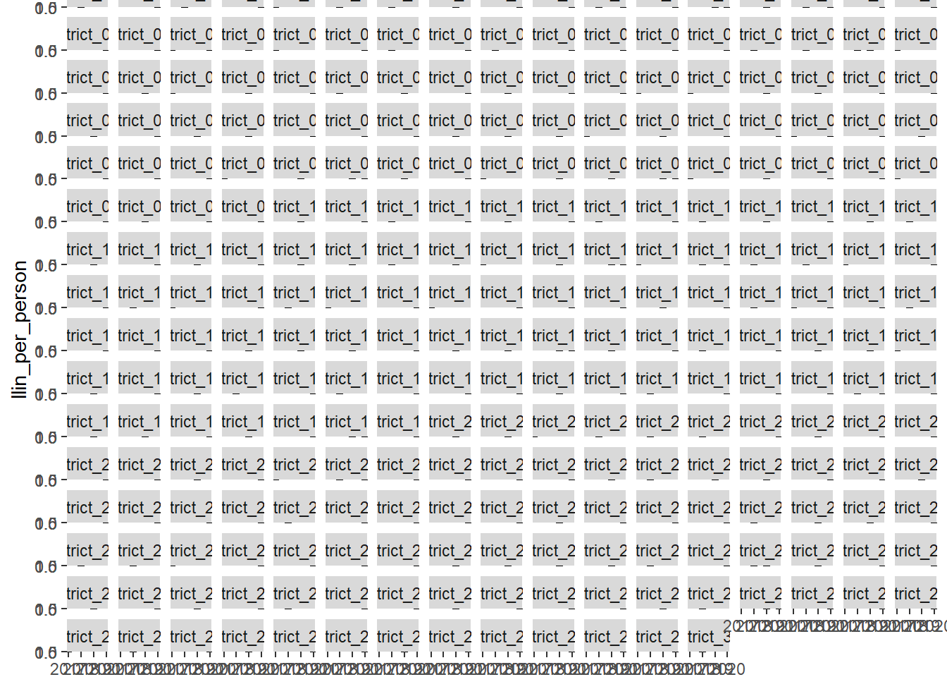
### convert mass LLIN data into long formatmass_llin_long<- mass_llin_dist |>pivot_longer(cols =contains("llin"),names_to ="year_txt", values_to ="llin") |>mutate(year =as.numeric(substr(year_txt,6,9))) |> dplyr::select(-year_txt)### convert population data into long formatpopulation_long<- population |>pivot_longer(cols =contains("pop"),names_to ="year_txt",values_to ="pop")|>mutate(year =as.numeric(substr(year_txt,5,8))) |> dplyr::select(-year_txt)### join the two and generate llin per person mllin_pop = mass_llin_long |>left_join(population_long,by =c("region","zone","district","year")) |>mutate(llin_per_person = llin/pop)### visualizemllin_pop|>filter(llin_per_person>0) |>ggplot(aes(x=year, y = llin_per_person)) +facet_wrap (~ district) +geom_point()
Mass distributions often assume two persons would use a single LLIN. In other words, 100% coverage would be achieved if a district gets LLIN about half its population. Thus, it would be somewhat curious if a district reports LLIN per person greater than 0.5, and even more suspicious if they report figures greater than 1. Note that the data quality issues can come from one or both of the two data sets used, mass LLIN and the population denominator.
Exercise 1: How many districts in the above example reported LLIN per person values greater than 1 in any year?
2.1.2Routine LLIN distribution data
In this exercise, we will look at an example of mock routine LLIN distribution data for the sample districts. This exercise assumes the LLIN data and accompanying population figures have been cleaned and verified for consistency and completeness.
First, let us load the necessary libraries.
library(tidyverse)library(lubridate)
We will read data on LLIN distribution through routine programs (EPI and ANC). We will further read the corresponding population data for each district.
Rows: 1200 Columns: 12
── Column specification ────────────────────────────────────────────────────────
Delimiter: ","
chr (3): region, zone, district
dbl (9): year, llins_epi_u6m, llins_epi_611m, llins_epi_1223m, llins_epi_245...

ℹ Use `spec()` to retrieve the full column specification for this data.
ℹ Specify the column types or set `show_col_types = FALSE` to quiet this message.
population<-read_csv("data/pop_2017_2020.csv")
Rows: 300 Columns: 7
── Column specification ────────────────────────────────────────────────────────
Delimiter: ","
chr (3): region, zone, district
dbl (4): pop_2017, pop_2018, pop_2019, pop_2020

ℹ Use `spec()` to retrieve the full column specification for this data.
ℹ Specify the column types or set `show_col_types = FALSE` to quiet this message.
We can visualize and verify if our data is consistent with the expectation. To do that we join the LLIN distribution datasets with the corresponding population data.
The following script does that by (a) converting the datasets into long format (b) joining them based on geographic units and years, and (c) generating LLINs per estimated population under five years old by assuming U5 population is roughly a fifth of the overall population.
### convert routine LLIN data into long formatroutine_llin_long<- routine_llin_dist |>pivot_longer(cols =contains("llin"),names_to ="program",values_to ="llin")### convert population data into long formatpopulation_long<- population |>pivot_longer(cols =contains("pop"),names_to ="year_txt", values_to ="pop") |>mutate(year =as.numeric(substr(year_txt,5,8))) |> dplyr::select(-year_txt)### join the two and generate llin per personrllin_pop <- routine_llin_long |>left_join(population_long,by =c("region","zone","district","year")) |>group_by(region, zone, district, year) |>summarise(rllin =sum(llin, na.rm=T),population =mean(pop)) |>ungroup() |>mutate(llin_per_u5 = rllin/population *5) # assuming U5 a fifth of pop.
`summarise()` has grouped output by 'region', 'zone', 'district'. You can
override using the `.groups` argument.
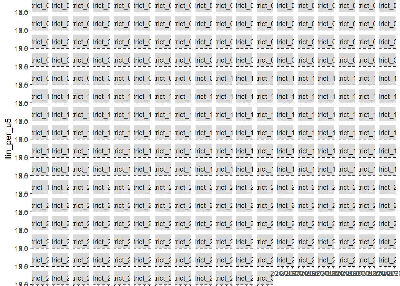
## visualizerllin_pop|>ggplot(aes(x=year, y = llin_per_u5)) +facet_wrap (~ district) +geom_point()
Unlike mass distributions, routine LLINs are distributed without consideration of the size of the population targeted. Rather, they are handed out during the visits by members of the population. However, we can have a broad assumption such as that the number of LLINs dispensed may not exceed the n time the population of under-five-year-old children. Data points flagged in this manner can also be subject to further scrutiny as part of the data cleaning process.
Exercise 2: How many districts in the above example reported routine LLIN per U5 population values greater than 5 in any year?
2.1.3Access to LLIN at the population level
Following LLIN distributions LLIN access as a result of the distribution in the year can be easily estimated. In the next script, we will bring both mass campaign and routine LLIN distribution data together and generate estimates of access to LLIN. In calculating access to LLIN at the population level, will assume one LLIN serves an average of 1.8 individuals in the population.
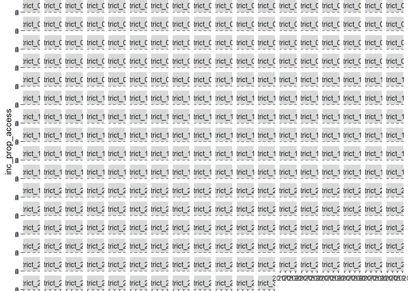
### increment to the proportion with access to LLINllin_access<- mllin_pop |>left_join(rllin_pop,by =c("region", "zone", "district", "year")) |>mutate(total_llin = llin + rllin) |>mutate(llin_per_person = total_llin/population) |>mutate(inc_prop_access = llin_per_person*1.8) |> dplyr::select(region, zone, district, year, total_llin, llin_per_person, inc_prop_access)## visualizellin_access|>ggplot(aes(x=year, y = inc_prop_access)) +facet_wrap (~ district) +geom_point()
Since access to LLIN is given in percentages, we can assume a maximum of 1, and districts with values beyond that may be flagged for further checking of their data.
Exercise 3: How many districts in the above example reported increment to proportion with access to LLIN of greater than 100% (>1.0) ?