DHIS2 Data cleaning

MACEPA, Data Fellowship Retreat

Important

All data, figures, and analyses are intended for educational purposes only and should not be used for decision-making, and have been adjusted or simulated to protect sensitive information. Do not use outputs from this project outside of the educational context!

This worksheet demonstrates basic principles, procedures, and steps to perform data cleaning on DHIS2 data. DHIS2 is widely used across countries to collect routine health data, including malaria, from health facilities up to national dashboards. However, analysts often encounter challenges such as:

• inconsistent names for geographies, health facilities, or data elements​

• missing, duplicated, or miscoded values​

• structural or format differences between datasets or reporting periods​

These issues can make it difficult to merge or compare data across sources and years, generate accurate visualizations and summaries​, and produce reliable insights for programmatic decision making.

In this worksheet, we will cover four major components of data cleaning as related to DHIS2:

• Structural cleaning

• Harmonization

• Geographic cleaning

• Outlier detection

We will begin by loading the necessary packages and a dataset prepared for this demonstration. The dataset is scrambled version of the DRC data, thus is not necessarily useful for any purpose outside this workshop.

1 Basic data cleaning

1.1 Loading and exploring data

# load libraries
library(tidyverse)
library(janitor)
library(lubridate)
library (stringi)

# load necessary data
dat<- read_csv("material/data/processed/df_malaria_scrambled_messy_DRC_hsv.csv")

Once we load the data,, we begin by explore the dataset’s different features: what are its dimensions?, what columns does it have? In particular, we would be trying to identify which columns are related to: geographies, time, data elements, and the value.

dim(dat)

[1] 594792     11

names (dat)

 [1] "orgunitlevel2"                     "orgunitlevel3"                    
 [3] "orgunitlevel4"                     "orgunitlevel5"                    
 [5] "organisationunitid"                "facility_type"                    
 [7] "d_9_6_paludisme_dcd_under_5_ans"   "d_9_6_paludisme_dcd_over_5_ans"   
 [9] "a_1_4_paludisme_grave_under_5_ans" "a_1_4_paludisme_grave_over_5_ans" 
[11] "periodid"                         

# #View(dat)

Question 1: From our exploration, identify which variables are related to:

• Time,

• Geographies,

• Health facility

• Data elements

1.2 Structural data cleaning

We will start by cleaning the column names:

dat<- dat |>
  janitor::clean_names()

names(dat)

 [1] "orgunitlevel2"                     "orgunitlevel3"                    
 [3] "orgunitlevel4"                     "orgunitlevel5"                    
 [5] "organisationunitid"                "facility_type"                    
 [7] "d_9_6_paludisme_dcd_under_5_ans"   "d_9_6_paludisme_dcd_over_5_ans"   
 [9] "a_1_4_paludisme_grave_under_5_ans" "a_1_4_paludisme_grave_over_5_ans" 
[11] "periodid"                         

It turns out, we did not need to use clean_names() as the data looks to have that done already.

1.3 Selecting only necessary variables

It’s good practice to remove variables that you don’t plan to use in your analysis.

# A tibble: 594,792 × 11
   orgunitlevel2    orgunitlevel3 orgunitlevel4 orgunitlevel5 organisationunitid
   <chr>            <chr>         <chr>         <chr>         <chr>             
 1 Bas Uele  Provi… Aketi  Zone … Aboso  Aire … Health Facil… SH8PSQ            
 2 Bas Uele  Provi… Poko  Zone d… Kana  Aire d… CHW_00002     BBOIUA            
 3 Bas Uele  Provi… Titule  Zone… Agemeto  Air… Health Facil… PEN35U            
 4 Bas Uele  Provi… Aketi  Zone … Ahaupa  Aire… Health Facil… V93905            
 5 Bas Uele  Provi… Viadana  Zon… Akpudu  Aire… Health Facil… K2L21Q            
 6 Bas Uele  Provi… Poko  Zone d… Amadi  Aire … Health Facil… J0GYJ4            
 7 Bas Uele  Provi… Bondo  Zone … Panzaka  Air… CHW_00007     OWYWJD            
 8 Bas Uele  Provi… Aketi  Zone … Andea  Aire … Health Facil… HD3K5D            
 9 Bas Uele  Provi… Titule  Zone… Andoma  Aire… Health Facil… O57K95            
10 Bas Uele  Provi… Ganga  Zone … Ngbandea  Ai… CHW_00010     VPJQS0            
# ℹ 594,782 more rows
# ℹ 6 more variables: facility_type <chr>,
#   d_9_6_paludisme_dcd_under_5_ans <dbl>,
#   d_9_6_paludisme_dcd_over_5_ans <dbl>,
#   a_1_4_paludisme_grave_under_5_ans <dbl>,
#   a_1_4_paludisme_grave_over_5_ans <dbl>, periodid <dbl>

Let’s remove facility_type as we don’t expect to use this variable

dat1<-
  dat |> dplyr::select(-facility_type)
  
names(dat1)

 [1] "orgunitlevel2"                     "orgunitlevel3"                    
 [3] "orgunitlevel4"                     "orgunitlevel5"                    
 [5] "organisationunitid"                "d_9_6_paludisme_dcd_under_5_ans"  
 [7] "d_9_6_paludisme_dcd_over_5_ans"    "a_1_4_paludisme_grave_under_5_ans"
 [9] "a_1_4_paludisme_grave_over_5_ans"  "periodid"                         

Note: It’s a good idea to remove data once we no longer need it - this keeps our workspace tidy.

rm(dat)

Question 2: How you you remove multiple variables?

1.4 Renaming columns

Let us have a look at the available columns now.

We will rename the following columns:

• orgunitlevel2 is not clear what it is: we want to change it to province

• orgunitlevel3 is not clear what it is: we want to change it to district

• orgunitlevel4: is not clear what it is: we want to change it to health_area

• orgunitlevel5 is not clear what it is: we want to change it to health_facility

• organisationunitud is too long and hard to memorize: we want to change it to hfid

dat1<- dat1 |>
  rename(hfid = organisationunitid,
         health_facility = orgunitlevel5,
         health_area = orgunitlevel4,
         district = orgunitlevel3,
         province = orgunitlevel2
         )

names(dat1)

 [1] "province"                          "district"                         
 [3] "health_area"                       "health_facility"                  
 [5] "hfid"                              "d_9_6_paludisme_dcd_under_5_ans"  
 [7] "d_9_6_paludisme_dcd_over_5_ans"    "a_1_4_paludisme_grave_under_5_ans"
 [9] "a_1_4_paludisme_grave_over_5_ans"  "periodid"                         

1.5 Changing to long format data

A clean dataset needs to have a single row for each observation. For this reason, we want to have a dataset in long format. For example, if we have a dataset that has columns for each data element, would want to change the format so that each data element has a unique row for each health facility- month.

The dataset we have is in wide format and we need to change the format to long so that each row has one observation only. But will also need to work on the names of the columns which are currently in French (in data harmonization section).

• “a_1_4_paludisme_grave_under_5_ans” = “Severe malaria cases among under 5 years”

• “a_1_4_paludisme_grave_over_5_ans” = “Severe malaria cases among age 5 years and above”

• “d_9_6_paludisme_dcd_under_5_ans” = “deaths due to malaria among under 5 years”

• “d_9_6_paludisme_dcd_over_5_ans” = “deaths due to malaria among age 5 years and above”

Let us change the format to long first.

We advise to make a new data frame if the changes you make to a data frame that mean it would not work if the code chunk was rerun. The following exercise is one such example. If we run the code twice (without following through all of the above steps and keeping the name as dat), we run into an error.

dat2<-
  dat1 |> 
  pivot_longer(cols = (contains("a_1") | contains("d_9")),
                       names_to = "data_type_fr",
                       values_to = "value") 

dat2 |> distinct(data_type_fr)

# A tibble: 4 × 1
  data_type_fr                     
  <chr>                            
1 a_1_4_paludisme_grave_under_5_ans
2 a_1_4_paludisme_grave_over_5_ans 
3 d_9_6_paludisme_dcd_under_5_ans  
4 d_9_6_paludisme_dcd_over_5_ans   

rm(dat1)

1.6 Split composite values

We now observe that data types have two things:

• the indicator and

• the age group

We need to split the column into two: and make sure one value. separate for the indicator and the age group.

We advise to make a new data frame if the changes you make to a data frame do not guarantee similar results when rerun multiple times. The following exercise is one such example. If we run the code twice (without following through all of the above steps and keeping the name as dat2), we run into an error.

dat3 <- 
  dat2 |>    
  mutate(data_type = case_when(str_detect(data_type_fr, "grave") ~ "severe_malaria",
                               str_detect(data_type_fr, "dcd") ~ "malaria_death"),
         age_group = case_when(str_detect(data_type_fr, "over_5") ~ "over_5",
                               str_detect(data_type_fr, "under_5") ~ "under_5"))  
rm(dat2) 

Lets check this worked! We’ll make sure the values and categories produce the same values

#new data elements
dat3 |>
  group_by(data_type, age_group) |>
  summarise(total = sum(value, na.rm=TRUE))    

# A tibble: 4 × 3
# Groups:   data_type [2]
  data_type      age_group   total
  <chr>          <chr>       <dbl>
1 malaria_death  over_5      10114
2 malaria_death  under_5     18978
3 severe_malaria over_5    2717855
4 severe_malaria under_5   2449271

# old data element
dat3 %>% group_by(data_type_fr) |>
  summarise(total = sum(value, na.rm=TRUE))

# A tibble: 4 × 2
  data_type_fr                        total
  <chr>                               <dbl>
1 a_1_4_paludisme_grave_over_5_ans  2717855
2 a_1_4_paludisme_grave_under_5_ans 2449271
3 d_9_6_paludisme_dcd_over_5_ans      10114
4 d_9_6_paludisme_dcd_under_5_ans     18978

Once we have the data_type values split into two columns, it’s easier to quickly add up all the malaria deaths

Let us remove the old column name (now split into two) before we proceed.

dat3 <-    dat3 |>
  dplyr::select (-contains("data_type_fr"))

2 Data harmonization

Harmonization bridges the gap between messy field data and standardized analytical data.​It ensures that our data:

• is consistent across indicators (variables) and values

• uses naming format that have standard structure

• Makes the data comparable across time and sources​

2.1 Standardizing date

the periodid column has a double numeric value. We want to change the value to to date format of “YYYY-MM-DD”.

Question 3:: Generate a new column with the name period by converting the periodid value into date format of “YYYY-MM_DD”

dat3<-    
  dat3 |>
  mutate(period = 
           lubridate::ymd(paste0(substr(periodid, 1,4), "-", substr(periodid, 5,6), "-01"))) |>
  dplyr::select(-periodid)  

##View(dat3)    

Question 4 : Generate a new column with the name year by extracting the year part of the variable period. Can you do similar to create a new column for month?

dat3<-    
  dat3 |>
  mutate(year = year(period))  

names(dat3)         

 [1] "province"        "district"        "health_area"     "health_facility"
 [5] "hfid"            "value"           "data_type"       "age_group"      
 [9] "period"          "year"           

We can easily make a facet_grid plot that shows the total for each data_type and age_group

dat3 |>   
  group_by(year, data_type, age_group) |>   
  summarise(total = sum(value, na.rm = T), .groups = "drop") |>
  ggplot (aes (x=factor(year), y = total)) +
  geom_col( fill = "tomato") +
  facet_grid(data_type ~ age_group, scale = "free_y") + 
  theme_bw()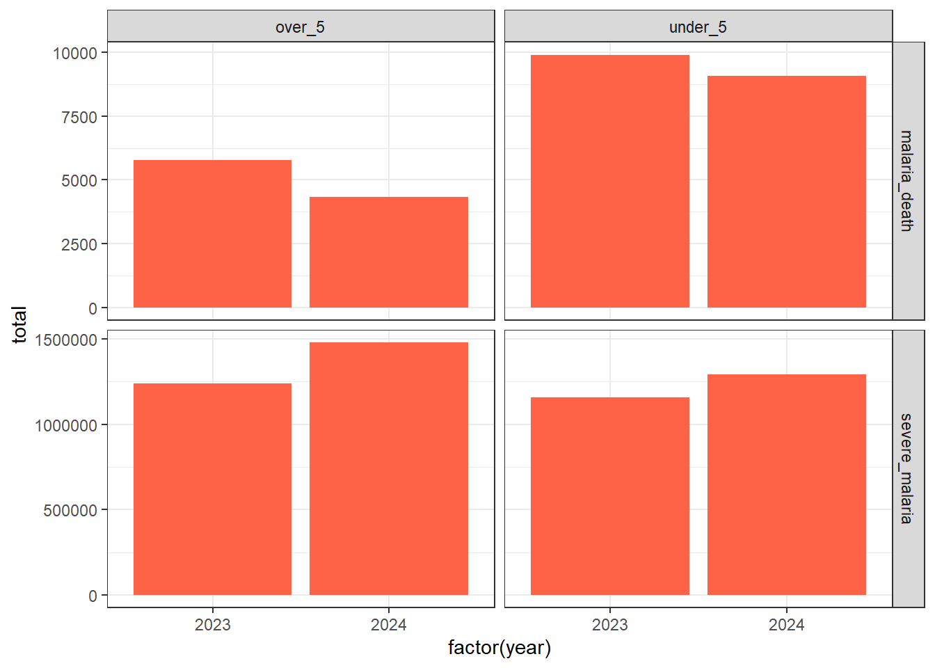

Question 5a: What does scale = “free_y” do?

Question 5b: How could we change this to have data_type on the top and age group on the side?

Question 6: Can you make a single plot for each data type with stacked bars showing the cases/deaths in each age group in a different colour?

3 Geographic cleaning

Here we want to use the shapefile as a reference dataset and join the DHIS2 data to the reference geographic names. To do that we will upload the shapefile first and extract reference names for province and health_zone.

3.1 Define a reference dataset for geographic names

drc_ref_names<- readRDS("material/data/raw/shapefiles/drc-admin2-clean-id.RDS") |>
  sf::st_drop_geometry() %>% 
  dplyr::select(province, health_zone)

names(drc_ref_names)
# we'll use the columns province and health_zone to match to

drc_ref_names |>
  distinct(province) %>% 
  nrow()

[1] 26

drc_ref_names |>
  distinct(province, health_zone) %>% 
  nrow()

[1] 519

There are 26 provinces and 519 districts that we need to match.

Lets start by using the quick-win data cleaning steps that we saw in the lecture this morning

3.2 Quick-win name cleaning

dat3 <- dat3 %>% 
  # Remove foreign characters (convert to ASCII, drop unconvertible)
  mutate(province = iconv(province, from = "UTF-8", to = "ASCII//TRANSLIT"),
         district = iconv(district, from = "UTF-8", to = "ASCII//TRANSLIT")) %>% 
  # Consistent capitalisation (we'll choose to use Title Case) %>% 
  mutate(province = str_to_title(province),
         district = str_to_title(district)) %>% 
  # Remove unwanted characters 
  # this uses regex (regular expression) to remove all "-", "_", "/"
  # (i never remember how to do these and always use chatGPT/google)
  mutate(province = str_replace_all(province, "[-_/]", " "),
         district = str_replace_all(district, "[-_/]", " ")) %>% 
    # this uses 'regex' to remove all brackets/parenthesis
    mutate(province = str_replace_all(province, "[\\(\\)]", ""),
         district = str_replace_all(district, "[\\(\\)]", "")) %>% 
  # remove trailing, leading white space, ensure only one space between words
  mutate(province = str_trim(province),
         district = str_trim(district),
         province = str_replace_all(province, "\\s+", " "),
         district = str_replace_all(district, "\\s+", " "))     

Now lets see how many non-matches there are for province first. anti_join is a really useful function for name matching - here it’s return all the entries of dat3 that do NOT have a match in the provinces in drc_ref_names.

3.3 Checking non-matches with anti_join

dat3 %>% anti_join(drc_ref_names, by = "province") %>% 
  distinct(province)

# A tibble: 26 × 1
   province               
   <chr>                  
 1 Bas Uele Province      
 2 Equateur Province      
 3 Haut Katanga Province  
 4 Kongo Central Province 
 5 Haut Lomami Province   
 6 Haut Uele Province     
 7 Lualaba Province       
 8 Lomami Province        
 9 Ituri Province         
10 Kasai Oriental Province
# ℹ 16 more rows

3.4 Manual fixes

So we see that there were 26 unjoined provinces!! It looks like the provinces all have the word ‘province’ in the name - lets remove these

dat4 <-
  dat3 |>
  # note also removing the whitespace before province
  mutate(province = str_remove(province, " Province"))

head(dat4)

# A tibble: 6 × 10
  province district  health_area health_facility hfid  value data_type age_group
  <chr>    <chr>     <chr>       <chr>           <chr> <dbl> <chr>     <chr>    
1 Bas Uele Aketi Zo… Aboso  Air… Health Facilit… SH8P…     4 severe_m… under_5  
2 Bas Uele Aketi Zo… Aboso  Air… Health Facilit… SH8P…     4 severe_m… over_5   
3 Bas Uele Aketi Zo… Aboso  Air… Health Facilit… SH8P…    NA malaria_… under_5  
4 Bas Uele Aketi Zo… Aboso  Air… Health Facilit… SH8P…    NA malaria_… over_5   
5 Bas Uele Poko Zon… Kana  Aire… CHW_00002       BBOI…    NA severe_m… under_5  
6 Bas Uele Poko Zon… Kana  Aire… CHW_00002       BBOI…    NA severe_m… over_5   
# ℹ 2 more variables: period <date>, year <dbl>

Now lets check again how many are unmatched

dat4 %>% anti_join(drc_ref_names, by = "province") %>% 
  distinct(province)

# A tibble: 1 × 1
  province 
  <chr>    
1 Maindombe

Now we see that there is one remaining unmatched province - lets take a look in the reference data to see what this is

drc_ref_names %>% 
  distinct(province) %>% 
  pull(province)

 [1] "Mongala"        "Ituri"          "Sud Kivu"       "Nord Ubangi"   
 [5] "Kinshasa"       "Kongo Central"  "Tanganyika"     "Kasai Central" 
 [9] "Tshopo"         "Nord Kivu"      "Kasai Oriental" "Maniema"       
[13] "Sud Ubangi"     "Sankuru"        "Haut Katanga"   "Kasai"         
[17] "Haut Lomami"    "Kwango"         "Lomami"         "Equateur"      
[21] "Bas Uele"       "Lualaba"        "Kwilu"          "Mai Ndombe"    
[25] "Haut Uele"      "Tshuapa"       

It looks like Mai Ndombe can be spelt with a space in the middle - lets fix this manually

dat4<-
  dat4 |>
  mutate(province = case_when (province =="Maindombe" ~ "Mai Ndombe",
                               TRUE ~ province))
  
## check if there are any more mismatches
dat4 %>% anti_join(drc_ref_names, by = "province") 

# A tibble: 0 × 10
# ℹ 10 variables: province <chr>, district <chr>, health_area <chr>,
#   health_facility <chr>, hfid <chr>, value <dbl>, data_type <chr>,
#   age_group <chr>, period <date>, year <dbl>

There are no more mismatches in the province name (indicated by having zero rows in our table of non-matches)

Now lets move onto district / health_zone matching

dat4 %>% anti_join(drc_ref_names, by = c("province", "district" = "health_zone")) %>% 
  distinct(province, district)

# A tibble: 519 × 2
   province district             
   <chr>    <chr>                
 1 Bas Uele Aketi Zone De Sante  
 2 Bas Uele Poko Zone De Sante   
 3 Bas Uele Titule Zone De Sante 
 4 Bas Uele Viadana Zone De Sante
 5 Bas Uele Bondo Zone De Sante  
 6 Bas Uele Ganga Zone De Sante  
 7 Bas Uele Ango Zone De Sante   
 8 Bas Uele Bili Zone De Sante   
 9 Bas Uele Likati Zone De Sante 
10 Bas Uele Buta Zone De Sante   
# ℹ 509 more rows

There are no matches again! (Indicated by having 519 in the dataframe of no-matches) It looks like these all have ‘Zone De Sante’ included

Lets remove this first and try again

dat4 <-
  dat4 |>
  # note also removing the whitespace before province
  mutate(district = str_remove(district, " Zone De Sante"))

head(dat4)

# A tibble: 6 × 10
  province district health_area  health_facility hfid  value data_type age_group
  <chr>    <chr>    <chr>        <chr>           <chr> <dbl> <chr>     <chr>    
1 Bas Uele Aketi    Aboso  Aire… Health Facilit… SH8P…     4 severe_m… under_5  
2 Bas Uele Aketi    Aboso  Aire… Health Facilit… SH8P…     4 severe_m… over_5   
3 Bas Uele Aketi    Aboso  Aire… Health Facilit… SH8P…    NA malaria_… under_5  
4 Bas Uele Aketi    Aboso  Aire… Health Facilit… SH8P…    NA malaria_… over_5   
5 Bas Uele Poko     Kana  Aire … CHW_00002       BBOI…    NA severe_m… under_5  
6 Bas Uele Poko     Kana  Aire … CHW_00002       BBOI…    NA severe_m… over_5   
# ℹ 2 more variables: period <date>, year <dbl>

Now lets try the anti_join again

dat4 %>% anti_join(drc_ref_names, by = c("province", "district" = "health_zone")) %>% 
  distinct(province, district)

# A tibble: 32 × 2
   province       district       
   <chr>          <chr>          
 1 Bas Uele       Bili           
 2 Equateur       Mampoko        
 3 Haut Katanga   Ruashi         
 4 Ituri          Mongbwalu      
 5 Ituri          Gety           
 6 Kongo Central  Muanda         
 7 Kongo Central  Massa          
 8 Kongo Central  Nsona Mpangu   
 9 Kasai Oriental Kabeya Kamwanga
10 Kasai Oriental Citenge        
# ℹ 22 more rows

3.5 Fuzzy name matching

There are 32 districts that are unmatched. One option would be to correct these manually like we did with the unmatched province. Another option is to employ fuzzy matching. Lets try that here

We will use the fuzzyjoin package to do these matches. We will further use the Jaro Winkler (“jw”) method in the stringdist_inner_join function to joining names based on their difference relative to their respective lengths.

For computational reasons, we want to narrow down our join to those that did no have matches.

library(fuzzyjoin)

# make a list of all the districts with no match (make sure to include the each 
# districts province)
no_match = dat4 %>% 
  anti_join(drc_ref_names, by = c("province", "district" = "health_zone")) %>% 
  distinct(province, district)

# this attempts to match districts based on 'similar' names
# We use the Jaro-Winkler method with provides a % difference, so 0 = identical
# here we just look at matches < 0.15, but you might need to increase this if
# no matches are returned 

new_name<- fuzzyjoin::stringdist_inner_join(
  no_match, drc_ref_names,
  by = c("province",
          "district" = "health_zone"),
  method = "jw",
  max_dist = 0.15,
  distance_col = "dist_jw"
) 

Looking at new_name we see there are now 38 rows, this is because there are some instances where multiple matches have been found for a district. Inspecting this, it looks like there is a discrepancy where in one dataset numbers are written i.e. 1, 2, and in the other they are I, Ii. This is an easy one to fix manually. Normally I’d add this to my ‘quick-fix’ code above and rerun, but for now I’ll just add it here.

# checking all the data that have multiple suggested matches
new_name %>% group_by(district) %>% 
  count() %>% 
  filter(n>=2)

# A tibble: 10 × 2
# Groups:   district [10]
   district           n
   <chr>          <int>
 1 Bili               2
 2 Kalamu 1           2
 3 Kalamu 2           2
 4 Lubunga            2
 5 Maluku 1           2
 6 Maluku 2           2
 7 Masina 1           2
 8 Masina 2           2
 9 Mont Ngafula 1     2
10 Mont Ngafula 2     2

dat4 <- dat4 %>% 
  mutate(district = str_replace(district, "2", "Ii"),
         district = str_replace(district, "1", "I"))

no_match = dat4 %>% anti_join(drc_ref_names, by = c("province", "district" = "health_zone")) %>% 
  distinct(province, district)

new_name2<- fuzzyjoin::stringdist_inner_join(
  no_match, drc_ref_names,
  by = c("province",
          "district" = "health_zone"),
  method = "jw",
  max_dist = 0.15,
  distance_col = "dist_jw"
) 

# the only 2 entries with multiple matches are now Bili and Lubunga
new_name2 %>% group_by(district) %>% 
  count() %>% 
  filter(n>=2)

# A tibble: 2 × 2
# Groups:   district [2]
  district     n
  <chr>    <int>
1 Bili         2
2 Lubunga      2

Lets manually inspect the corrections to see if we think they are correct.

All the suggestions look good to me - lets just replace them in the main data. If there were remaining issues, they could be corrected manually or you could choose to use the suggestion with the lower J-W distance.

# firstly make a flag in the new_name2 dataset that can be used
# after joining to the main data to identify which names
# need to be replaced
new_name2 <- new_name2 %>% 
  mutate(flag_no_name_match = 1)

dat5 <- dat4 %>% 
  left_join(new_name2, by = c("province" = "province.x",
                              "district")) %>% 
  # if the flag is 1, then we replace the 'incorrect' district name
  # with the correct health_zone name from drc_ref_names
  mutate(district = if_else(!is.na(flag_no_name_match), health_zone, district)) %>% 
  # now lets remove these unwanted columns to keep the data tidy 
  dplyr::select(-c(province.y, health_zone, district.dist_jw, province.dist_jw, dist_jw))


# now lets double check this has all worked correctly

dat5 %>% anti_join(drc_ref_names, by = c("province", "district" = "health_zone")) %>% 
  distinct(province, district)

# A tibble: 2 × 2
  province       district
  <chr>          <chr>   
1 Equateur       Mampoko 
2 Kasai Oriental Citenge 

Here , we can see that there are two more district names that did not even fuzzy_join due to exceeding maximum distance requirement of 0.15 we set in the function. Lets look for these manually…

3.6 Manual fixes pt.2

# lets see if we can find a district that looks like "Mampoko" 
drc_ref_names %>% filter(province == "Equateur")

   province     health_zone
1  Equateur         Lotumbe
2  Equateur        Mbandaka
3  Equateur         Bomongo
4  Equateur         Ingende
5  Equateur         Monieka
6  Equateur          Djombo
7  Equateur        Lukolela
8  Equateur         Wangata
9  Equateur         Bolomba
10 Equateur         Bolenge
11 Equateur Lilanga Bobangi
12 Equateur          Bikoro
13 Equateur         Makanza
14 Equateur           Irebu
15 Equateur Lolanga Mampoko
16 Equateur           Iboko
17 Equateur       Basankusu
18 Equateur          Ntondo

# We spotted "Lolanga Mampoko" - this could be the match,
# but first let's double check that we don't already have a district with this name
dat5 %>% filter(district == "Lolanga Mampoko")

# A tibble: 0 × 11
# ℹ 11 variables: province <chr>, district <chr>, health_area <chr>,
#   health_facility <chr>, hfid <chr>, value <dbl>, data_type <chr>,
#   age_group <chr>, period <date>, year <dbl>, flag_no_name_match <dbl>

# Nope, so lets amend dat5

dat5 <- dat5 %>% 
  mutate(district = case_when(district == "Mampoko" ~ "Lolanga Mampoko",
                              TRUE ~ district))

Question 9: Can you find a match for Citenge and fix it in the code? Can you conduct a final check to see if all the names are correctly matched?

It is now time to save our cleaned dataset so far.

write_csv(dat5 |>
            dplyr::select (-flag_no_name_match) , "material/data/processed/df_malaria_cleaned_DRC_has_age_group_hsv.csv")

4 Outlier detection and correction

An outlier is a data point that is unusually different from the rest of the observations — it lies far outside the general pattern of your data. Data collection processes are prone to outliers, and DHIS2 is no exception. In DHIS2, outlier detection is best done at month-health facility level.

It is important to properly explore and correct outliers, otherwise, when we conduct analyses using the data we can get misleading patterns

4.1 Robust z-score approach

A standard z-score approach is to call a value an outlier if it is some number of standard deviations greater or less than the mean of the indicator (at the HF level). However, this approach can result in big biases as sometimes the ouliers are many orders of magnitude larger than the rest of the data, which can really skew the mean and standard deviation.

Our ‘robust z-score approach’ involves using the mean and SD of the middle 80% (ranked by size) of the data to determine if a value can be considered an outlier. For each health facility, we will generate mean and standard deviation (SD) of the middle 80% values for each of the two data elements in our dataset: malaria deaths and severe malaria.

4.2 Determining a threshold value

The threshold value is the number of standard deviations away from the mean that constitutes an outlier. It requires careful thought and consideration to select an appropriate value of this for your data.

In this exercise, we will initially experiment with the value of 10, before looking at alternative values.

# threshold multiplier of the SD
n_sds = 10

# start by aggregating over both age groups
dat6 <- dat5 |>
  group_by(province, district, health_facility, hfid, data_type, period) |>
  summarise(value = sum(value, na.rm=T), .groups = "drop") 

# calculate the mean and sd (of the middle 80%) - two indicators  each HF
# and calculate the max value an indicator can be before it's
# classified as an outlier (mean_80 + n_sds*sd_80)

outlier_vals <- dat6|>
  filter(!is.na(value)) |>
  filter(value > 0) |>
  group_by(province, district, health_facility, hfid, data_type) |> 
  arrange(value) |> 
  mutate(rank = row_number()) |> 
  # keep values with in the 10th and 90th percentiles (to reduce effects of outliers)
  filter(rank > n() * 0.1, rank <= n() * 0.9) |> # Filter the middle 80%
  summarise(mean_value = mean(value, na.rm=TRUE),
            sd_value = sd(value, na.rm=TRUE),
            outlier_max_value = mean_value + n_sds*sd_value) %>% 
  ungroup()

##View(dat6)

4.3 Determining outliers based on threshold value

## unusually high values -  identify outliers
dat_with_outlier <- 
  dat6 |>
  # bring in overall mean and sd
  left_join(outlier_vals, by = c("province", "district", "health_facility", "hfid", 
                               "data_type")) |>
  ## identify unusually high values ( > overall mean + 10 sd)
  mutate(outlier = case_when(value > outlier_max_value ~ 1,
                                    is.na(value) | is.na(sd_value) ~ 0,
                                   TRUE ~ 0))

##View(dat_with_outlier)

look_at_outliers <- dat_with_outlier %>% filter(outlier == 1)

4.4 Manual changes to outlier rules

There are lots of very small values that are being considered outliers. One might choose to just manually determine that any value under, say, 50 is not an outlier

dat_with_outlier <- dat_with_outlier %>% 
  mutate(outlier = if_else(value < 50, 0, outlier))

4.5 Visualizing outliers

Let start by looking at some of the rows classified as outliers

Visualization is an important step in outlier ditections and correction process. We use it to :

• select appropriate threshold multiplier by visualizing and making sure the detection is catching clear outliers

• See how good our correction has been

Visualize a sample of health facilities to see how good our outlier detection approach performed.

in this example, we generate a random sample of HF from among those that had an outlier identified.

# find all hf's that have >= 1 outlier
outlier_hfs<- dat_with_outlier |> 
  filter(outlier==1) |> 
  distinct(province, district, hfid) 

ssize = 42
set.seed(123)

# lets generate 4 sets of 42 HFs to sample over
# often we'd want to look at a lot more than this 
all_samp <- sample(outlier_hfs$hfid, 42*4, replace = FALSE)

samp1 <- all_samp[1:42]
samp2 <- all_samp[43:84]
samp3 <- all_samp[84:126]
samp4 <- all_samp[127:168]

We will then extract data for the selected random HFs for visualization. As severe malaria and malaria deaths are on very different scales, it’ll be easier to look at them separately. We’ll look at severe malaria here

 dat_with_outlier |> filter(hfid %in% samp1) |>
  filter(data_type == "severe_malaria") |>
    ggplot() +
    geom_line(aes(x = period, y = value, color = data_type)) +
    geom_point(aes(x = period, y = value, color = data_type), size = 0.5) +
    geom_point(aes(x = period, y = value, size = outlier, color = data_type), shape = 1) +
    facet_wrap(vars(health_facility), scale="free_y") +
    theme_bw()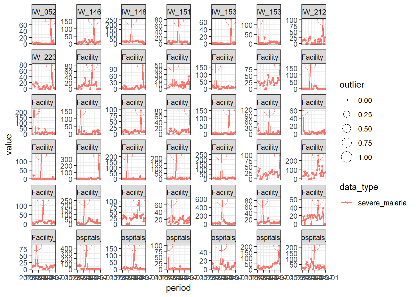

Question 8: (a) Looking at the sample health facilities above what do you think about our method? Can you make this plot for all 4 samples of hfids?

(b) Do you think it captured all extreme values we think are outliers?

(c) Did it select value that do not seem outliers?

(d)Try a different threshold multiplier and see how good your catches will be.

(e)Can you make similar plots to look at outliers in the mortality data?

4.6 Outlier correction

Finally , we want to correct the detected outliers by replacing them with the mean of the middle 80 percent we developed earlier.

# correct identified outlier values} 

dat_corrected<- dat_with_outlier |> 
  mutate(value_corrected = case_when (outlier ==1 ~ mean_value,
                                      TRUE ~ value))

Finally, we would visualize the corrected outlier to do a before- and - after comparison.

# dat_corrected |> left_join(hf_smp, by = c("district", "health_facility")) |>
#     filter(!is.na(row_num )) |> 
#     mutate(outlier_ind = ifelse(value > thresh_value, 1, NA)) |>
#     ggplot() +
#     geom_line(aes(x = period, y = value_corrected, color = data_type)) +
#     geom_point(aes(x = period, y = value_corrected, color = data_type), size = 0.5) +
#     geom_point(aes(x = period, y = value_corrected, size = outlier_ind, color = data_type), shape = 1) +
#     facet_wrap(vars(health_facility), scale="free_y") +
#     theme_bw()

Question 9: (a) Looking at the corrections and the original outlier do you think the correction was realistic? (b) Do you think it did better or worse than when there was outlier?

Question 10: Assume we are detecting outliers for routine malaria cases data that includes tests, confirmed, and presumed cases. Are there things we should be cautious about beyond using the threshold to determine outliers? What are they?

It is now time to save our cleaned dataset.

dat_out<- dat_corrected |>
  dplyr::select(province, district, health_facility, hfid, data_type, age_group, period, value, value_corrected)

write_csv(dat_out, "material/data/processed/df_malaria_cleaned_DRC_hsv.csv")