Welcome to the first lesson in our series on analyzing spatial data in R, with a focus on malaria in sub-Saharan Africa. Spatial data, information tied to a specific location, is incredibly valuable for understanding disease patterns, targeting interventions, and evaluating public health programs. Whether you’re mapping malaria incidence, analyzing access to insecticide-treated nets (ITNs), or optimizing resource allocation, understanding spatial data is crucial.
This lesson will cover:
Types of Spatial Data: Raster and Vector
Geographic Projections: Why they matter and how to handle them.
Essential R Packages: sf, terra, and ggplot2. We’ll also introduce malariaAtlas!
Practical Examples: Applying these concepts to malaria-related data using the malariaAtlas package.
5.2 Types of Spatial Data
Spatial data comes in two main forms:
Raster Data: Think of this as a grid of cells, like a digital photograph. Each cell holds a value representing a specific characteristic at that location. Common examples include:
Satellite Imagery: Land cover, vegetation indices (NDVI), temperature, precipitation.
Elevation Data: Digital Elevation Models (DEMs).
Gridded Climate Data: Temperature, rainfall.
Population Data: Gridded population counts or densities are crucial for calculating rates (e.g., malaria cases per 1000 people). Examples include datasets from WorldPop (https://www.worldpop.org/) and the Gridded Population of the World (GPW).
Modelled Malaria Incidence Surfaces: These are predictive maps of malaria risk, often generated using statistical models that incorporate environmental, socioeconomic, and demographic factors. The Malaria Atlas Project (https://malariaatlas.org/) is a primary source for these surfaces.
In the context of malaria, raster data provides valuable insights into ecological suitability, environmental conditions, population distribution, and disease risk. For example, a high-resolution population raster overlaid with a malaria incidence raster can help identify high-risk populations and prioritize interventions.
Example: Here’s an example of a raster visualizing population density:
WorldPop Population density map
Vector Data: Represents spatial features as points, lines, or polygons.
Points: Individual locations, such as health facilities, households surveyed, or locations of mosquito traps.
Lines: Roads, rivers, or migration routes. Useful for assessing access to healthcare or movement patterns.
Polygons: Areas like administrative boundaries (countries, districts), land parcels, or areas of specific land use (e.g., rice paddies, urban areas). Essential for calculating rates and performing spatial joins.
For malaria analysis, vector data can represent administrative units for calculating malaria rates, locations of health facilities, or areas receiving specific interventions. Shapefiles are the most common way to store vector data.
Shapefiles: A Deeper Dive
Shapefiles, traditionally associated with ESRI (Environmental Systems Research Institute), are a ubiquitous format for storing vector data. However, it’s essential to understand that a “shapefile” isn’t a single file. It’s a collection of files with the same base name but different extensions. At a minimum, an ESRI shapefile requires these files:
.shp: The main file that stores the geometry (the coordinates of the points, lines, or polygons).
.shx: An index file that speeds up spatial queries.
.dbf: A database file (in dBase format) that stores the attribute data associated with each feature.
.prj: A projection file that defines the coordinate system used in the shapefile. (Important! Always check this!)
Sometimes you’ll also see files like .sbn and .sbx (spatial index files) or .xml (metadata).
When sharing a shapefile, you must share all these associated files together. If you only provide the .shp file, the data is incomplete and will likely not load properly.
Alternative Vector Formats:
While shapefiles are common, other vector formats exist, including:
GeoJSON (.geojson): A text-based format using JavaScript Object Notation (JSON) to represent geographic features. It’s increasingly popular due to its human-readable format and ease of use in web applications. sf can read and write GeoJSON files.
GeoPackage (.gpkg): An open, standards-based format for storing geospatial vector data in a single SQLite database file. It’s becoming a preferred format due to its simplicity and efficiency. sf also supports GeoPackage.
Example: Here’s an example of a vector polygon dataset:
Imagine trying to flatten an orange peel onto a flat surface. It’s impossible without distortion. The Earth is a sphere (more accurately, a geoid), and representing it on a flat map (in R or anywhere else) requires a projection.
Why Projections Matter: Different projections distort different properties (area, shape, distance, direction). Choosing the right projection is crucial for accurate measurements and analyses.
Coordinate Reference Systems (CRS): A CRS defines how geographic coordinates (latitude and longitude) are related to a flat map. It includes both the datum (a reference point for the Earth’s shape and position) and the projection itself.
Common CRSs:
WGS 84 (EPSG:4326): A widely used geographic CRS based on latitude and longitude. Often the default for data downloaded online. Good for displaying global data, but distances and areas are distorted.
UTM (Universal Transverse Mercator): Divides the Earth into zones, each with its own projection. Good for measuring distances and areas within a specific zone. Needs to be chosen based on the area of interest. For example, a large area in Eastern Africa might use UTM Zone 37S or 37N (check a UTM zone map!).
Africa Albers Equal Area Conic (EPSG:102022): A projected CRS designed to minimize area distortion across the African continent. Useful when comparing areas of different regions.
Checking and Transforming Projections in R: You’ll often need to check the CRS of your data and transform it to a more suitable one for your analysis.
Matching CRSs: Shapefiles and Coordinate Lists
A common challenge arises when you have spatial data in different formats, such as a shapefile for administrative boundaries and a CSV file containing the locations of health facilities (latitude and longitude). To accurately map these datasets together, you must ensure they share the same CRS.
Here’s a typical workflow:
Determine the CRS of the Shapefile: Use st_crs(your_shapefile) (we’ll show you how to load shapefiles in the R examples) to identify the CRS of your shapefile. Note the EPSG code (e.g., 4326, 32637, 102022).
Create an sf Object from the Coordinate List: Assuming your CSV file has columns named longitude and latitude, use st_as_sf() (we’ll show you how to do this in the R examples) to convert it into an sf object. Crucially, specify the CRS when creating the object. You’ll need to load your CSV data into R first and then transform it to a special object.
Transform the Coordinate List (if necessary): If the CRS of the new object does not match the CRS of your administrative boundary shapefile, use st_transform() (again, to be demonstrated in a code example) to transform it to the correct CRS.
Verify the Transformation: After the transformation, always double-check the CRS of the transformed object using st_crs() to ensure it matches the shapefile’s CRS.
Important Considerations:
Assumptions: It’s vital to know the CRS of your coordinate list. Don’t assume it’s WGS 84. If you’re unsure, contact the data provider or consult the data’s documentation. Making incorrect assumptions about the CRS can lead to significant mapping errors.
Unit Consistency: When performing spatial analysis (e.g., calculating distances), ensure all your data is in a projected CRS with units in meters or kilometers. Geographic CRSs (like WGS 84) use degrees, which are not suitable for distance calculations.
Example: Here’s an example showing how coordinates with the wrong coordinate system look when plotted with shapefile data:
Let’s introduce the key R packages we’ll be using.
sf (Simple Features): This is the modern standard for working with vector data in R. It efficiently handles shapefiles, geodatabases, and other vector formats. It seamlessly integrates with the tidyverse.
terra: A powerful package for working with raster data. It is designed to be a replacement for the older raster package, offering increased speed and efficiency. It is closely integrated with the sf package for vector data.
ggplot2: A versatile and widely-used package for creating visually appealing and informative maps and plots. It works beautifully with both sf and terra objects.
malariaAtlas: A package that provides access to a wealth of malaria-related data, including survey data, raster layers of malaria incidence and prevalence, and shapefiles of administrative boundaries. It’s a fantastic resource for malaria researchers.
tidyverse: A collection of R packages that share an underlying design philosophy, grammar, and data structures. We’ll be using the dplyr package for data manipulation, and the tidyr package for data wrangling.
tidyterra: Extends the functionality of ggplot2 to the terra package.
5.5 Practical Examples in R
Now, let’s apply these concepts to a practical example related to malaria in sub-Saharan Africa, using the malariaAtlas package to obtain data.
# Install the packages if you haven't already# install.packages(c("sf", "terra", "ggplot2", "malariaAtlas", "tidyverse", "tidyterra"))# Load the packageslibrary(sf)
Warning: package 'sf' was built under R version 4.3.3
Linking to GEOS 3.11.2, GDAL 3.8.2, PROJ 9.3.1; sf_use_s2() is TRUE
library(terra)
terra 1.7.55
library(malariaAtlas)
Warning: package 'malariaAtlas' was built under R version 4.3.3
Loading required package: ggplot2
Warning: package 'ggplot2' was built under R version 4.3.3
Registered S3 method overwritten by 'malariaAtlas':
method from
autoplot.default ggplot2
library(tidyverse)
Warning: package 'tidyr' was built under R version 4.3.3
Warning: package 'readr' was built under R version 4.3.3
── Conflicts ────────────────────────────────────────── tidyverse_conflicts() ──
✖ tidyr::extract() masks terra::extract()
✖ dplyr::filter() masks stats::filter()
✖ dplyr::lag() masks stats::lag()
ℹ Use the conflicted package (<http://conflicted.r-lib.org/>) to force all conflicts to become errors
library(tidyterra)
Warning: package 'tidyterra' was built under R version 4.3.3
Registered S3 method overwritten by 'tidyterra':
method from
autoplot.SpatRaster malariaAtlas
Attaching package: 'tidyterra'
The following object is masked from 'package:stats':
filter
5.5.1 Getting Administrative Boundaries with malariaAtlas
# Select a country - Let's stick with Ethiopiacty ="Ethiopia"# Get the district shapefile (admin level 2)adm2 <-getShp(cty, admin_level ="admin2")
Loading ISO 19139 XML schemas...
Loading ISO 19115 codelists...
Please Note: Because you did not provide a version, by default the version being used is 202403 (This is the most recent version of admin unit shape data. To see other version options use function listShpVersions)
Start tag expected, '<' not found
# Print the first few rows of the data framehead(adm2)
Simple feature collection with 6 features and 16 fields
Geometry type: MULTIPOLYGON
Dimension: XY
Bounding box: xmin: 35.1156 ymin: 5.6004 xmax: 39.4539 ymax: 12.3047
Geodetic CRS: WGS 84
iso admn_level name_0 id_0 type_0 name_1 id_1 type_1
1 ETH 2 Ethiopia 10000850 Country Amhara 10313856 Region
2 ETH 2 Ethiopia 10000850 Country Sidama 868130572 Region
3 ETH 2 Ethiopia 10000850 Country SNNP 10313355 Region
4 ETH 2 Ethiopia 10000850 Country SNNP 10313355 Region
5 ETH 2 Ethiopia 10000850 Country SNNP 10313355 Region
6 ETH 2 Ethiopia 10000850 Country Oromia 10316246 Region
name_2 id_2 type_2 name_3 id_3 type_3
1 Lake Tana 868128071 Water Body NA NA NA
2 Lake Awasa 868128081 Water Body NA NA NA
3 Sheka 10016531 Zone NA NA NA
4 Gamo 868128083 Zone NA NA NA
5 Amaro 10016516 Zone NA NA NA
6 North Shewa (OR) 10016504 Zone NA NA NA
source geometry country_level
1 Ethiopia CSA and BoFED 2020 MULTIPOLYGON (((37.6035 12.... ETH_2
2 Ethiopia CSA and BoFED 2020 MULTIPOLYGON (((38.482 7.09... ETH_2
3 Ethiopia CSA and BoFED 2020 MULTIPOLYGON (((35.5207 7.8... ETH_2
4 Ethiopia CSA and BoFED 2020 MULTIPOLYGON (((37.2744 6.7... ETH_2
5 Ethiopia CSA and BoFED 2020 MULTIPOLYGON (((38.0884 5.7... ETH_2
6 Ethiopia CSA and BoFED 2020 MULTIPOLYGON (((38.7529 10.... ETH_2
getShp(): A function from the malariaAtlas package that downloads the administrative boundaries shapefile for the specified country and admin level. Admin level 2 generally refers to districts or similar sub-national units.
head(): Shows the first few rows of the data, allowing us to explore the attributes associated with each district.
st_crs(): Confirms the Coordinate Reference System of the shapefile. Notice the EPSG code.
The ggplot code creates a basic map of the districts. theme_void() removes unnecessary map elements for a cleaner look.
5.5.2 Obtaining and Mapping Malaria Survey Data
# Get the malaria prevalence survey datapr <-getPR(country = cty, species ="BOTH")
Please Note: Because you did not provide a version, by default the version being used is 202406 (This is the most recent version of PR data. To see other version options use function listPRPointVersions)
Start tag expected, '<' not found
Warning: The `sourcedata` argument of `isAvailable_pr()` is deprecated as of
malariaAtlas 1.6.0.
ℹ The argument 'sourcedata' has been deprecated. It will be removed in the next
version. It has no meaning.
ℹ The deprecated feature was likely used in the malariaAtlas package.
Please report the issue at
<https://github.com/malaria-atlas-project/malariaAtlas/issues>.
Please Note: Because you did not provide a version, by default the version being used is 202406 (This is the most recent version of PR data. To see other version options use function listPRPointVersions)
Confirming availability of PR data for: Ethiopia...
PR points are available for Ethiopia.
Attempting to download PR point data for Ethiopia ...
Start tag expected, '<' not found
Data downloaded for Ethiopia.
# Inspect the first few rowshead(pr)
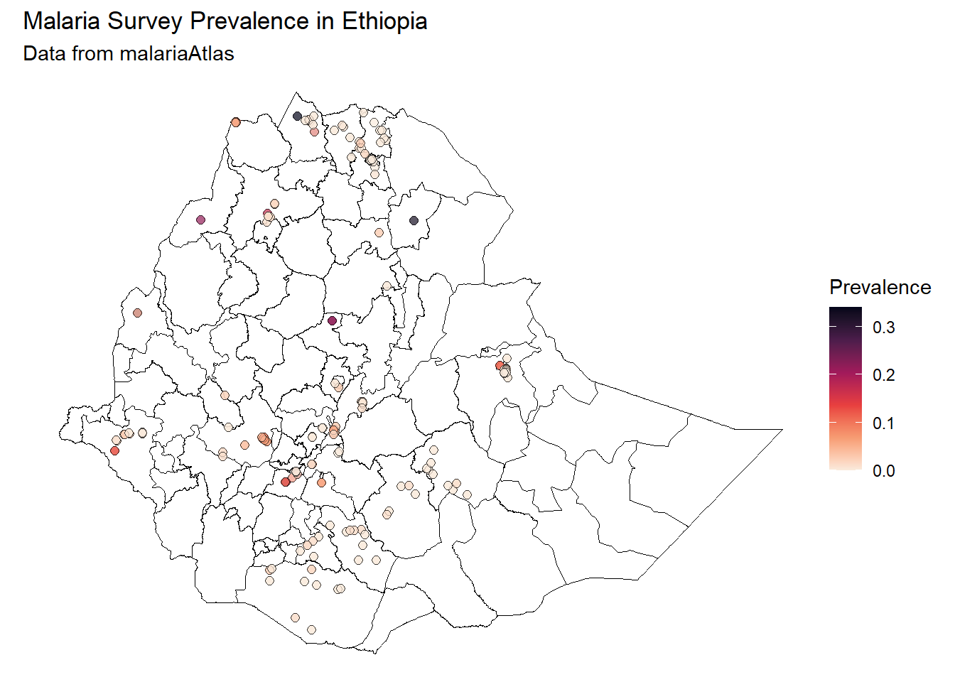
dhs_id site_id site_name latitude longitude rural_urban
7 <NA> 6694 Dole School 5.90141 38.94115 UNKNOWN
9 <NA> 10320 Langano 7.51600 38.77800 UNKNOWN
12 <NA> 8017 Gongoma School 6.31747 39.83618 UNKNOWN
15 <NA> 12873 Buriya School 7.56736 40.75210 UNKNOWN
18 <NA> 12260 Chobo 3 7.89960 34.45080 UNKNOWN
21 <NA> 21446 Mekele, Quiha & Aynalem 13.47600 39.50200 UNKNOWN
country country_id continent_id month_start year_start month_end year_end
7 Ethiopia ETH Africa 6 2009 6 2009
9 Ethiopia ETH Africa 4 2003 4 2003
12 Ethiopia ETH Africa 6 2009 6 2009
15 Ethiopia ETH Africa 6 2009 6 2009
18 Ethiopia ETH Africa 9 1989 10 1989
21 Ethiopia ETH Africa 9 1993 12 1993
lower_age upper_age examined positive pr species method
7 4.0 15 110 0 0.0000000 P. falciparum Microscopy
9 4.0 14 89 0 0.0000000 P. falciparum Microscopy
12 4.0 15 108 0 0.0000000 P. falciparum Microscopy
15 4.0 15 63 0 0.0000000 P. falciparum Microscopy
18 0.0 99 108 14 0.1296296 P. falciparum Microscopy
21 0.5 5 2080 0 0.0000000 P. falciparum Microscopy
rdt_type pcr_type malaria_metrics_available location_available
7 <NA> <NA> TRUE TRUE
9 <NA> <NA> TRUE TRUE
12 <NA> <NA> TRUE TRUE
15 <NA> <NA> TRUE TRUE
18 <NA> <NA> TRUE TRUE
21 <NA> <NA> TRUE TRUE
permissions_info
7 <NA>
9 <NA>
12 <NA>
15 <NA>
18 <NA>
21 <NA>
citation1
7 Ashton, RA, Kefyalew, T, Tesfaye, G, Pullan, RL, Yadeta, D, Reithinger, R, Kolaczinski, JH and Brooker, S (2011). <b>School-based surveys of malaria in Oromia Regional State, Ethiopia: a rapid survey method for malaria in low transmission settings.</b> <i>Malaria Journal</i>, <b>10</b>(1):25
9 Legesse, M. and Erko, B. (2004). <b>Prevalence of intestinal parasites among school children in a rural area close to the southeast of Lake Langano, Ethiopia.</b> <i>Ethiopian Journal of Health Development</i>, <b>18</b>(2):116-120
12 Ashton, RA, Kefyalew, T, Tesfaye, G, Pullan, RL, Yadeta, D, Reithinger, R, Kolaczinski, JH and Brooker, S (2011). <b>School-based surveys of malaria in Oromia Regional State, Ethiopia: a rapid survey method for malaria in low transmission settings.</b> <i>Malaria Journal</i>, <b>10</b>(1):25
15 Ashton, RA, Kefyalew, T, Tesfaye, G, Pullan, RL, Yadeta, D, Reithinger, R, Kolaczinski, JH and Brooker, S (2011). <b>School-based surveys of malaria in Oromia Regional State, Ethiopia: a rapid survey method for malaria in low transmission settings.</b> <i>Malaria Journal</i>, <b>10</b>(1):25
18 Nigatu, W., Abebe, M. and Dejene, A. (1992). <b><i>Plasmodium vivax</i> and <i>P. falciparum</i> epidemiology in Gambella, south-west Ethiopia.</b> <i>Tropical Medicine and Parasitology</i>, <b>43</b>(3):181-5
21 Adish, A.A., Esrey, S.A., Gyorkos, T.W. and Johns, T. (1999). <b>Risk factors for iron deficiency anaemia in preschool children in northern Ethiopia.</b> <i>Public Health Nutrition</i>, <b>2</b>(3):243-52
citation2 citation3
7 <NA> <NA>
9 <NA> <NA>
12 <NA> <NA>
15 <NA> <NA>
18 <NA> <NA>
21 <NA> <NA>
# Summarize the number of surveys.nrow(pr)
[1] 2794
# Convect survey data to sf object and match projection to adm2 shapefile# Note: missing coordinates must be removed before converting to sfpr_sf <- pr |>filter(!is.na(longitude) &!is.na(latitude) &!is.na(pr)) |>st_as_sf(coords =c("longitude", "latitude"), crs =st_crs(adm2))# Plot data using ggplotggplot() +geom_sf(data = adm2, fill =NA, color ="black", linewidth =0.1) +geom_sf(data = pr_sf, aes(fill = pr), shape =21, alpha =0.7, size =2) +scale_fill_viridis_c(option ="F", direction =-1, name ="Prevalence") +labs(title =paste("Malaria Survey Prevalence in", cty),subtitle ="Data from malariaAtlas") +theme_void()
Explanation:
getPR(): Retrieves malaria prevalence survey data for the specified country. The species = "BOTH" argument ensures we get data for all malaria species.
head(pr): Displays the first few rows of the pr data frame, showing the structure of the survey data (longitude, latitude, prevalence, etc.).
pr |> summarise(N = length(unique(survey_id))): This code uses tidyverse syntax to calculate the number of unique surveys in the data.
filter(!is.na(longitude) & !is.na(latitude) & !is.na(pr)): Removes rows with missing longitude, latitude, or prevalence values to avoid errors when creating the spatial object. This is critical!
st_as_sf(): Converts the data frame to an sf object, using the longitude and latitude columns as coordinates. The crs = st_crs(adm2) argument ensures the survey data is in the same coordinate system as the administrative boundaries.
The ggplot code overlays the survey points on the map of districts, with the color of the points representing the malaria prevalence. shape = 21 creates points with both a fill and an outline, and alpha = 0.7 makes the points slightly transparent to see underlying features.
<GMLEnvelope>
....|-- lowerCorner: 3.4011 32.9999 "2000-01-01T00:00:00"
....|-- upperCorner: 14.8942 47.9862 "2020-01-01T00:00:00"Start tag expected, '<' not found
# Plot the raster and shapefile using ggplotggplot() +geom_spatraster(data = inc) +geom_sf(data = adm2, fill =NA, color ="black", linewidth =0.1) +scale_fill_viridis_c(option ="F", direction =-1,name ="Incidence", na.value ="transparent") +labs(title =paste("Malaria Incidence in", cty),subtitle ="Data from malariaAtlas") +theme_void()
Explanation:
getRaster(): Downloads a raster dataset from the Malaria Atlas Project (MAP). The dataset_id specifies the raster layer we want (in this case, global Plasmodium falciparum incidence rate). The shp = adm2 argument crops the raster to the extent of the administrative boundaries, which saves memory and processing time. The shp argument also ensures that the raster data have the same CRS as the provided shapefile.
geom_spatraster: Plots raster data objects that are of the terra class spatRaster, in ggplot.
scale_fill_viridis_c(): Sets the color gradient for the raster data.
The ggplot code displays the malaria incidence raster overlaid on the district boundaries. na.value = "transparent" makes the background (areas with no data) transparent, allowing the map underneath to show through.
5.6 Challenge Questions/Exercises
Explore Different Countries: Modify the cty variable to analyze malaria data for a different country in sub-Saharan Africa (e.g., “Nigeria”, “Kenya”, “Uganda”). Run the code to generate maps for that country. What are some key differences in malaria prevalence or incidence compared to Ethiopia?
Different Administrative Levels: Experiment with different admin_level arguments in getShp() (e.g., admin_level = "admin1" for regions/provinces). How does the granularity of the map change?
Filter Survey Data: Filter the pr data frame to include only surveys conducted in a specific year or a specific region. Create a map showing only the filtered survey data.
Change Color Scales: Experiment with different color palettes in scale_fill_viridis_c(). Try other options like "A", "B", "C", etc., and explore reverse the ordering of the colour scale by using direction = 1. Which color scale do you find most effective for visualizing malaria prevalence and incidence?
Save the map: Save the last map as a png file using the ggsave() function.