6  Practical Example: Fixing coordinate data

6.1 Loading Packages

For these packages, if we have already installed them we can just load them using the “library()” command. If not, copy the name of the package into an “install.packages(”packagename”)” command to install them from CRAN.

library(sf)

Warning: package 'sf' was built under R version 4.3.3

Linking to GEOS 3.11.2, GDAL 3.8.2, PROJ 9.3.1; sf_use_s2() is TRUE

library(raster)

Loading required package: sp

library(tidyverse)

Warning: package 'ggplot2' was built under R version 4.3.3

Warning: package 'tidyr' was built under R version 4.3.3

Warning: package 'readr' was built under R version 4.3.3

── Attaching core tidyverse packages ──────────────────────── tidyverse 2.0.0 ──
✔ dplyr     1.1.4     ✔ readr     2.1.5
✔ forcats   1.0.0     ✔ stringr   1.5.1
✔ ggplot2   3.5.1     ✔ tibble    3.2.1
✔ lubridate 1.9.3     ✔ tidyr     1.3.1
✔ purrr     1.0.2     

── Conflicts ────────────────────────────────────────── tidyverse_conflicts() ──
✖ tidyr::extract() masks raster::extract()
✖ dplyr::filter()  masks stats::filter()
✖ dplyr::lag()     masks stats::lag()
✖ dplyr::select()  masks raster::select()
ℹ Use the conflicted package (<http://conflicted.r-lib.org/>) to force all conflicts to become errors

library(zoo)

Attaching package: 'zoo'

The following objects are masked from 'package:base':

    as.Date, as.Date.numeric

library(broom)

Warning: package 'broom' was built under R version 4.3.3

library(stringr)
library(ggpmisc)

Warning: package 'ggpmisc' was built under R version 4.3.3

Loading required package: ggpp

Warning: package 'ggpp' was built under R version 4.3.3

Registered S3 methods overwritten by 'ggpp':
  method                  from   
  heightDetails.titleGrob ggplot2
  widthDetails.titleGrob  ggplot2

Attaching package: 'ggpp'

The following object is masked from 'package:ggplot2':

    annotate

Warning in .recacheSubclasses(def@className, def, env): undefined subclass
"ndiMatrix" of class "replValueSp"; definition not updated

library(ggforce)
library(purrr)
library(dplyr)
library(rio)

Warning: package 'rio' was built under R version 4.3.3

6.2 Loading in necessary files

Our shapefile can be found in the data fellowship common folder. Just adjust the filepath to use your own username before the Box section of the filepath.

# You may need to adjust the filepath
usr <- Sys.info()[7]
district_shp <- readRDS(paste0("C:/Users/", usr,"/Box/Data fellowship program planning/Data fellowship common folder/dataset for practice/zambia_districts.RDS"))

#use your shapefile to make an outline of the country boundaries
bnd <- district_shp %>% rmapshaper::ms_dissolve() %>% st_geometry()
bnd_coords <- st_coordinates(district_shp)[,1:2] %>% as.data.frame %>% setNames(c("x", "y"))

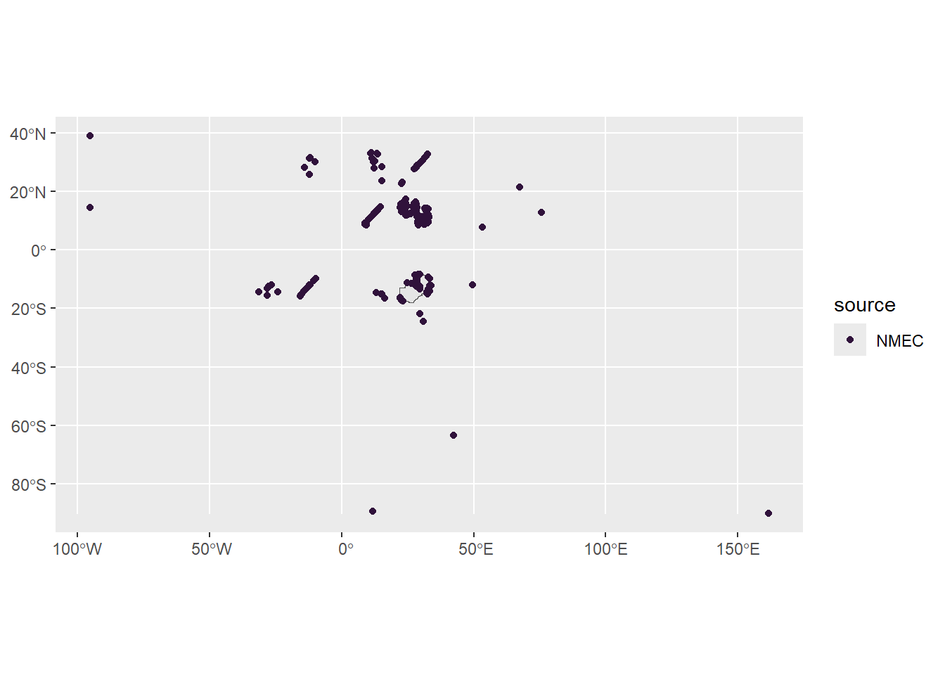
Currently this script uses health facility location data from the Zambia NMEC instance of DHIS2.

#use your own username here in place of "wsheahan"
nmec <- readRDS(paste0("C:/Users/", usr,"/Box/Data fellowship program planning/Data fellowship common folder/dataset for practice/zambia_facility_locations.RDS"))

6.3 Geocorrections Code

outside_boundary <- function(src, return_sf = FALSE, cmbl = nmec){
  
  suppressMessages(
    sf_out <- cmbl %>%
      filter(source %in%{{src}},
             !is.na(lon)) %>%
      st_as_sf(coords = c("lon", "lat"), crs = st_crs(bnd)) %>%
      filter(!st_intersects(geometry, bnd, sparse = FALSE))
  )
  
  tbl_out <- sf_out %>%
    mutate(lon = unlist(map(geometry,1)),
           lat = unlist(map(geometry,2))) %>%
    st_drop_geometry() %>%
    dplyr::select(org_unit_uid, lon, lat, everything())
  
  if(return_sf == T) {return(sf_out)} else {return(tbl_out)}
}

The outside_boundary function returns a list of all points in our file where the lat and lon are outside of our defined boundary shapefile (bnd)

outside_boundary("NMEC")

Warning: Using one column matrices in `filter()` was deprecated in dplyr 1.1.0.
ℹ Please use one dimensional logical vectors instead.

# A tibble: 707 × 13
   org_unit_uid   lon   lat org_unit_level parent_name         province district
   <chr>        <dbl> <dbl>          <int> <chr>               <chr>    <chr>   
 1 yNiDP74JNgJ   28.2  12.5              5 co Mufulira Clinic… Copperb… Mufulira
 2 XJOHbY24Bpd   28.2  12.5              5 co 14 Miles Health… Copperb… Mufulira
 3 MBYbQfbwqxz   28.2  12.5              5 co 14 Miles Health… Copperb… Mufulira
 4 aUqmlb5Vdzt   28.2  12.5              5 co 14 Miles Health… Copperb… Mufulira
 5 d856aHh17ap   28.2  12.5              5 co Mufulira Clinic… Copperb… Mufulira
 6 obZ0ZT9wk3K   28.1  13.6              5 co Nampamba Rural … Copperb… Mpongwe 
 7 x2Rr0NkLyN0   28.1  13.6              5 co Nampamba Rural … Copperb… Mpongwe 
 8 mC0OrY85VmX   28.1  13.6              5 co Nampamba Rural … Copperb… Mpongwe 
 9 XbCN4P6bTEY   24.8  14.8              5 we Luena Camp Hosp… Western  Kaoma   
10 QI0SjGZ9u0J   24.8  14.8              5 we Luena Camp Hosp… Western  Kaoma   
# ℹ 697 more rows
# ℹ 6 more variables: short_name <chr>, name <chr>, created <chr>,
#   source <chr>, c_month <chr>, c_year <chr>

we can use ggplot to visually confirm that these points are not where they are supposed to be

ggplot() +
  geom_sf(data = bnd) +
  geom_sf(data = outside_boundary("NMEC", return_sf = T),
          aes(color = source)) +
  scale_color_viridis_d(option = "H")

mispecified_location <- function(src, by = "province", cmbl = nmec) {
  
  suppressMessages(
    out <- cmbl %>%
      filter(source == {{src}},
             !is.na(lon)) %>%
      st_as_sf(coords = c("lon", "lat"), crs = st_crs(bnd)) %>%
      st_join(district_shp) %>%
      mutate(lon = unlist(map(geometry,1)),
             lat = unlist(map(geometry,2))) %>%
      st_drop_geometry() %>%
      dplyr::select(org_unit_uid, lon, lat,
                    province, geo_province,
                    district, geo_district,
                    everything())
  )
  if(by == "province") {return(filter(out, province != geo_province))}
  if(by == "district") {return(filter(out, district != geo_district))}
}

mispecified_location("NMEC", by = "province")

# A tibble: 286 × 18
   org_unit_uid   lon   lat province geo_province district     geo_district
   <chr>        <dbl> <dbl> <chr>    <chr>        <chr>        <chr>       
 1 zcPf4NedM57   24.5 -14.0 Western  Northwestern Lukulu       Mufumbwe    
 2 J6bFDOwxKLx   24.5 -14.0 Western  Northwestern Lukulu       Mufumbwe    
 3 Bewp3Y613qp   24.5 -14.0 Western  Northwestern Lukulu       Mufumbwe    
 4 AnK50NuUn1M   26.8 -15.3 Southern Central      Itezhi-tezhi Mumbwa      
 5 Eusw992Dk0H   25.1 -16.4 Southern Western      Kazungula    Mulobezi    
 6 DEaMRBXpa5H   25.1 -17.2 Southern Western      Kazungula    Mwandi      
 7 n3vwfWM2frv   26.6 -15.3 Southern Central      Itezhi-tezhi Mumbwa      
 8 b9ZkT5JVZeq   27.8 -15.7 Southern Lusaka       Mazabuka     Kafue       
 9 q3ToaprI7Lg   26.6 -15.6 Central  Southern     Mumbwa       Itezhi-tezhi
10 Ch6ck1OVbvz   28.0 -15.4 Central  Lusaka       Shibuyunji   Chilanga    
# ℹ 276 more rows
# ℹ 11 more variables: org_unit_level <int>, parent_name <chr>,
#   short_name <chr>, name <chr>, created <chr>, source <chr>, c_month <chr>,
#   c_year <chr>, pop_grid3_2022 <dbl>, area_km2 <dbl>, reported_district <chr>

mispecified_location("NMEC", by = "district")

# A tibble: 1,615 × 18
   org_unit_uid   lon   lat province     geo_province district   geo_district
   <chr>        <dbl> <dbl> <chr>        <chr>        <chr>      <chr>       
 1 cZhbmotVmjD   31.1 -14.5 Eastern      Eastern      Petauke    Nyimba      
 2 zcPf4NedM57   24.5 -14.0 Western      Northwestern Lukulu     Mufumbwe    
 3 J6bFDOwxKLx   24.5 -14.0 Western      Northwestern Lukulu     Mufumbwe    
 4 tdZNyirEls7   22.8 -16.5 Western      Western      Shang'ombo Sioma       
 5 fET5Q3mqIIx   22.8 -16.5 Western      Western      Shang'ombo Sioma       
 6 Vdri40jbFvG   22.8 -16.5 Western      Western      Shang'ombo Sioma       
 7 xmF8B7xkbkU   28.2 -15.5 Lusaka       Lusaka       Chilanga   Lusaka      
 8 sEjZ3MhIYAE   28.2 -15.5 Lusaka       Lusaka       Chilanga   Lusaka      
 9 Tnr0CSfapvM   28.2 -15.5 Lusaka       Lusaka       Chilanga   Lusaka      
10 fcq9iqgC52e   23.7 -13.9 Northwestern Northwestern Kabompo    Zambezi     
# ℹ 1,605 more rows
# ℹ 11 more variables: org_unit_level <int>, parent_name <chr>,
#   short_name <chr>, name <chr>, created <chr>, source <chr>, c_month <chr>,
#   c_year <chr>, pop_grid3_2022 <dbl>, area_km2 <dbl>, reported_district <chr>

Misspecified_location does something similar. With this function we can build a dataset of all the points that we believe are in the “wrong” district and then shift their coordinates as needed.

mis_loc_chw <- mispecified_location("NMEC", by = "district")

#Shift coordinates
shift_coord <- function(org_coords, valid_coords) {
  
  # input_class <- class(org_coords)
  org_coords <- as.data.frame(org_coords)
  n <- nrow(org_coords)
  x <- y <- numeric(length = n)
  
  for(i in 1:n){
    new_loc <-  valid_coords[which.min(
      (valid_coords[,1]-org_coords[i,1])^2 +
        (valid_coords[,2]-org_coords[i,2])^2),]
    
    x[i] <- new_loc[1]
    y[i] <- new_loc[2]
  }
  out <- cbind(x, y)
  
  # If input is a dataframe, return a dataframe with the same column names
  if(class(org_coords) == "data.frame") {
    out <- as.data.frame(out)
    names(out) <- names(org_coords)
  }
  
  return(out)
}

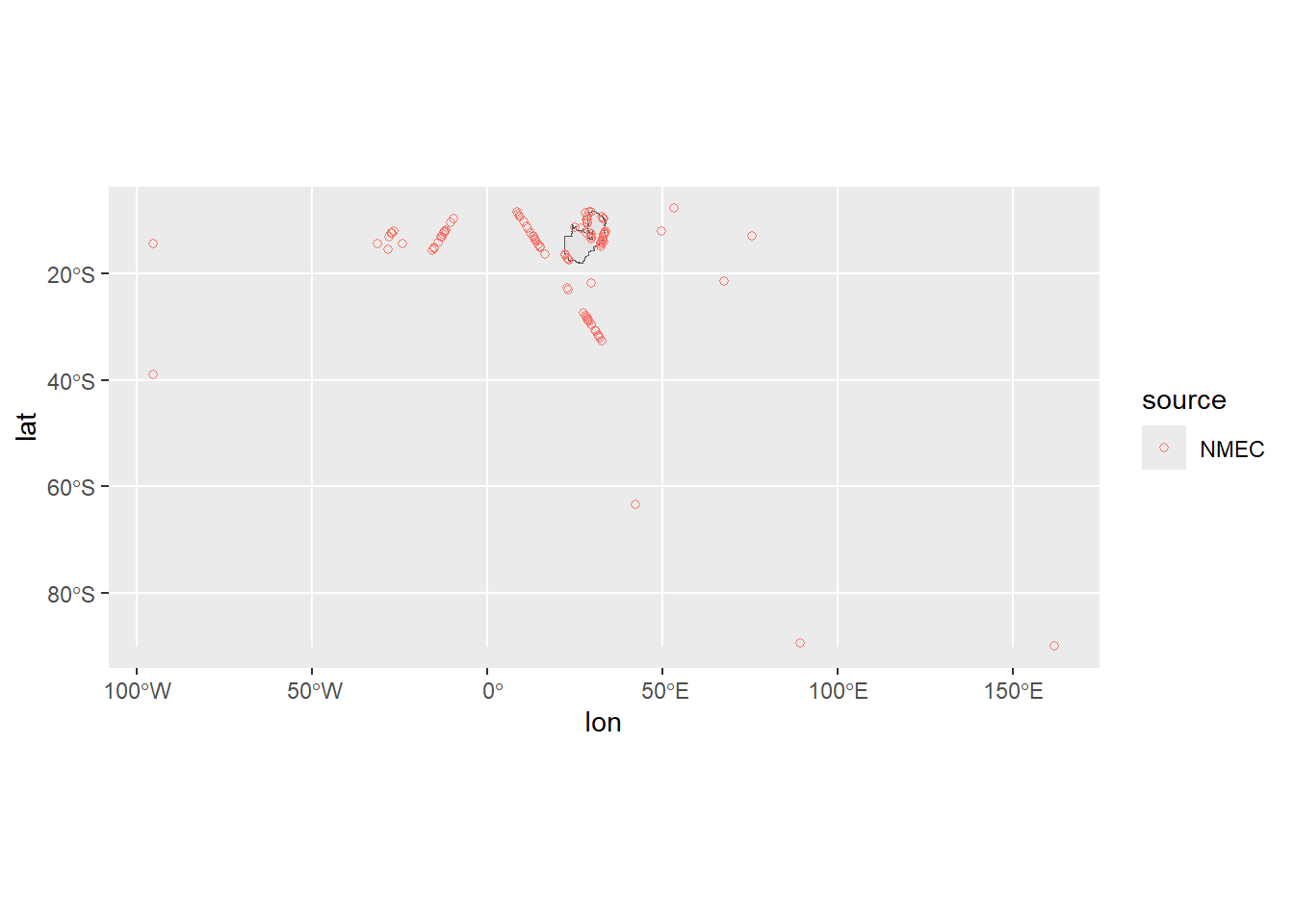
These are some standard geocorrections for common errors such as lat/lon being 0, having a - or + flipped in the lat/lon, or when lat/lon are flipped it basically checks to see if fixing those common issues would put the point back into the bnd area where it belongs.

std_geocorrections <- outside_boundary("NMEC") %>%
  mutate(
    new_lon = case_when(
      # Set 0 to NA
      lon == 0 ~ NA_real_,
      
      # Fixing signs
      between(-lon, min(bnd_coords$x), max(bnd_coords$x)) &
        between(-lat, min(bnd_coords$y), max(bnd_coords$y)) ~ -lon,
      
      # Lat and lon flipped
      between(lon, min(bnd_coords$y), max(bnd_coords$y)) &
        between(lat, min(bnd_coords$x), max(bnd_coords$x)) ~ lat,
      
      # Otherwise leave unchanged
      TRUE ~ lon),
    
    new_lat = case_when(
      # Set 0 to NA
      lat == 0 ~ NA_real_,
      
      # Fixing signs
      between(-lon, min(bnd_coords$x), max(bnd_coords$x)) &
        between(-lat, min(bnd_coords$y), max(bnd_coords$y)) ~ -lat,
      
      # Lat and lon flipped
      between(lon, min(bnd_coords$y), max(bnd_coords$y)) &
        between(lat, min(bnd_coords$x), max(bnd_coords$x)) ~ lon,
      
      # Only lat is negative
      # between(!lat, min(bnd_coords$y), max(bnd_coords$y)) &
      # between(-lat, min(bnd_coords$y), max(bnd_coords$y)) ~ -lat,
      lat > 0 ~ -lat,
      
      # Otherwise leave unchanged
      TRUE ~ lat)
    
  ) %>%
  mutate(
    # Double flips (sign and x,y)
    new_lon2 = case_when(
      between(-new_lon, min(bnd_coords$y), max(bnd_coords$y)) ~ -new_lat,
      TRUE ~ new_lon
    ),
    new_lat2 = case_when(
      between(-new_lat, min(bnd_coords$x), max(bnd_coords$x)) ~ -new_lon,
      TRUE ~ new_lat
    )
  )

#EDIT: Dropped in fix to new_lon/lat fields (Check)
std_geocorrections <- std_geocorrections %>%
  mutate(lon = new_lon2, lat = new_lat2) %>%
  dplyr::select(-c(new_lon, new_lon2, new_lat, new_lat2))

We can rerun outside_boundary on the list of “fixed” points to figure out which ones are still outside the boundary.

we can visually check these again, we should have a visibly smaller number of unfixed points than before.

ggplot(unfixed_geo) +
  geom_sf(data = bnd) +
  geom_point(aes(lon, lat, color = source), shape = 21)

# This are corrected and can be swapped back in
std_geo_fixed <- anti_join(std_geocorrections, unfixed_geo)

Joining with `by = join_by(org_unit_uid, lon, lat, org_unit_level, parent_name,
province, district, short_name, name, created, source, c_month, c_year)`

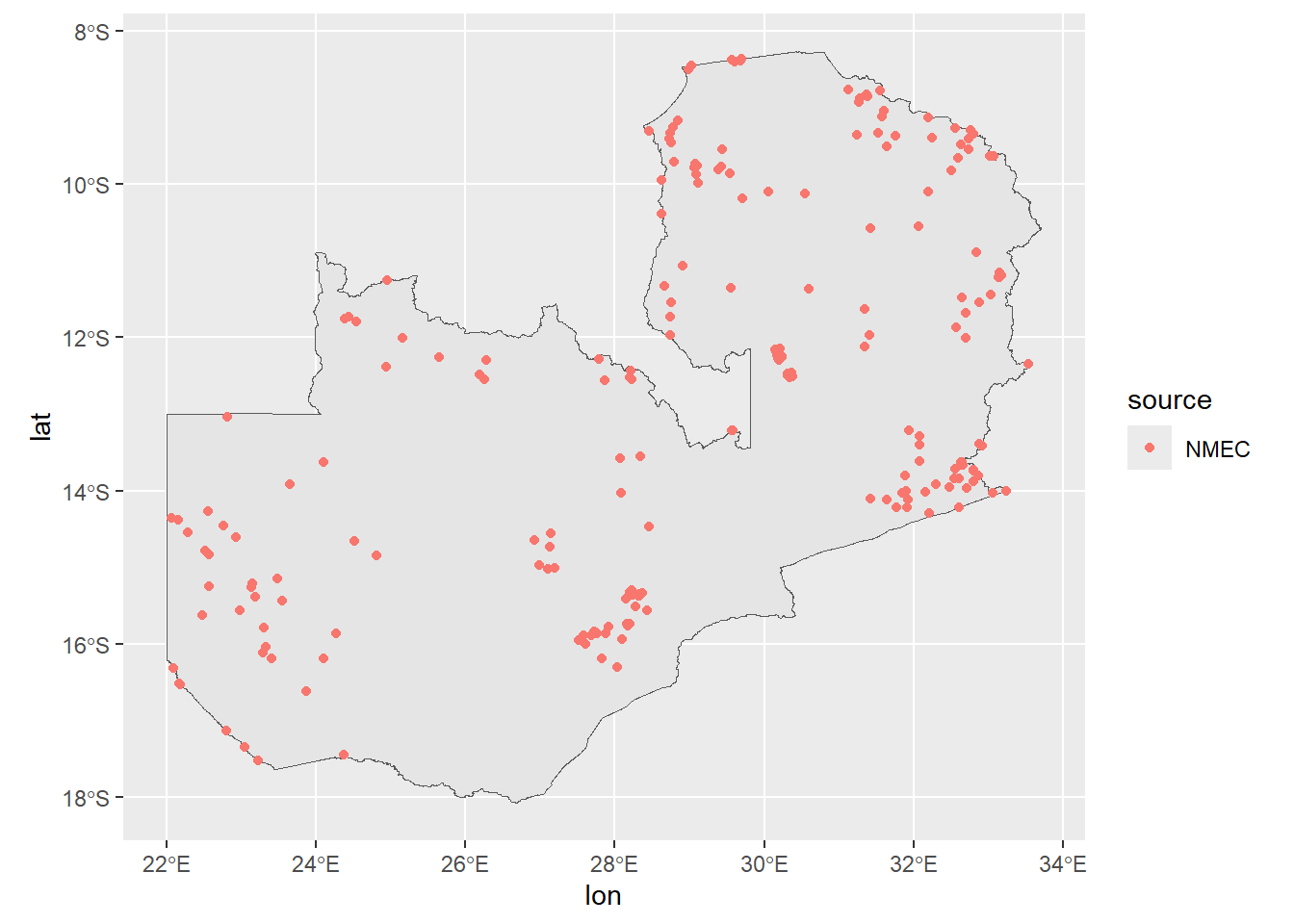
#Move bordering coordinates (<= 1 km) inside country
near_boundary <- outside_boundary("NMEC", cmbl = std_geocorrections, return_sf = T) %>%
  mutate(near_bnd = st_is_within_distance(., bnd, dist = units::as_units(1, "km"), sparse = F)[,1]) %>%
  mutate(lon = unlist(map(geometry,1)),
         lat = unlist(map(geometry,2))) %>%
  st_drop_geometry() %>%
  filter(near_bnd == TRUE) %>%
  mutate(new_lon = unlist(shift_coord(dplyr::select(., lon, lat), bnd_coords)[,1]),
         new_lat = unlist(shift_coord(dplyr::select(., lon, lat), bnd_coords)[,2]),
         lon = new_lon, lat = new_lat) %>%
  dplyr::select(-c(near_bnd, new_lon, new_lat))

#join the corrected locations with the ones we just nudged inside
corrected_geolocations <- bind_rows(std_geo_fixed, near_boundary)

#visualize to make sure they are all inside the boundary
ggplot(corrected_geolocations) +
  geom_sf(data = bnd) +
  geom_point(aes(lon, lat, color = source))

We then want to set our remaining out-of-bound locations to NA and then visually establish that our final list of geocorrected entries are all within the bounds of our geography.

unfixed_locations <- outside_boundary("NMEC") %>%
  anti_join(corrected_geolocations, by = c("org_unit_uid" = "org_unit_uid", "source" = "source")) %>%
  mutate(lon = NA_real_, lat = NA_real_)

geocorrect_combined_list <- nmec %>%
  # Remove original entries
  anti_join(outside_boundary("NMEC")) %>%
  bind_rows(corrected_geolocations, unfixed_locations)

Joining with `by = join_by(org_unit_uid, org_unit_level, lon, lat, parent_name,
province, district, short_name, name, created, source, c_month, c_year)`

corrected_geolocations %>%
  dplyr::select(org_unit_uid, source, new_lon = lon, new_lat = lat) %>%
  left_join(dplyr::select(nmec, org_unit_uid, source, old_lon = lon, old_lat = lat))

Joining with `by = join_by(org_unit_uid, source)`

# A tibble: 570 × 6
   org_unit_uid source new_lon new_lat old_lon old_lat
   <chr>        <chr>    <dbl>   <dbl>   <dbl>   <dbl>
 1 yNiDP74JNgJ  NMEC      28.2   -12.5    28.2    12.5
 2 XJOHbY24Bpd  NMEC      28.2   -12.5    28.2    12.5
 3 MBYbQfbwqxz  NMEC      28.2   -12.5    28.2    12.5
 4 aUqmlb5Vdzt  NMEC      28.2   -12.5    28.2    12.5
 5 d856aHh17ap  NMEC      28.2   -12.5    28.2    12.5
 6 obZ0ZT9wk3K  NMEC      28.1   -13.6    28.1    13.6
 7 x2Rr0NkLyN0  NMEC      28.1   -13.6    28.1    13.6
 8 mC0OrY85VmX  NMEC      28.1   -13.6    28.1    13.6
 9 XbCN4P6bTEY  NMEC      24.8   -14.8    24.8    14.8
10 QI0SjGZ9u0J  NMEC      24.8   -14.8    24.8    14.8
# ℹ 560 more rows

geo_corrected_nmec <- corrected_geolocations %>%
  dplyr::select(org_unit_uid, source, new_lon = lon, new_lat = lat) %>%
  left_join(dplyr::select(nmec, org_unit_uid, source, old_lon = lon, old_lat = lat)) %>%
  filter(source == "NMEC")

Joining with `by = join_by(org_unit_uid, source)`

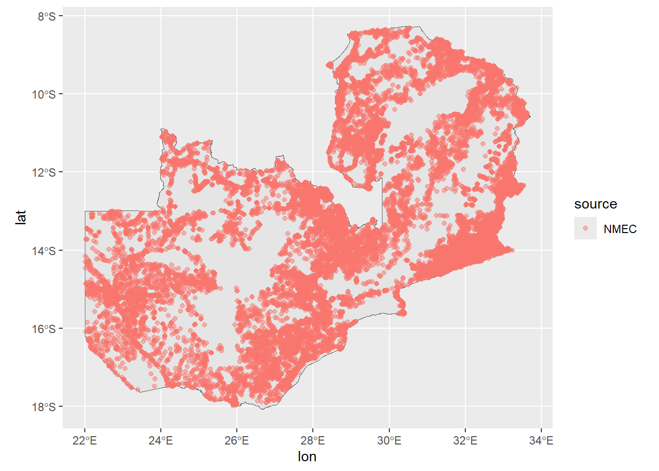
#get a finalized list of corrected chws
gc_nmec <- geocorrect_combined_list %>% filter(source == "NMEC") %>% 
  filter(org_unit_level == 5)


#Plot the points to make sure none remaining outside Zambia
ggplot(gc_nmec) +
  geom_sf(data = bnd) +
  geom_point(aes(lon, lat, color = source), alpha = 0.5) 

Warning: Removed 2385 rows containing missing values or values outside the scale range
(`geom_point()`).